
Incentivized Resume Rating: Eliciting Employer
Preferences without Deception
Judd B. Kessler, Corinne Low, and Colin D. Sullivan
∗
April 19, 2019
Abstract
We introduce a new experimental paradigm to evaluate employer prefer-
ences, called Incentivized Resume Rating (IRR). Employers evaluate resumes
they know to be hypothetical in order to be matched with real job seekers,
preserving incentives while avoiding the deception necessary in audit studies.
We deploy IRR with employers recruiting colle ge seniors from a prestigious
school, randomizing human capital characteristics and demographics of hypo-
thetical candidates. We measure both employer preferences for candidates and
employer b e li e fs about the likelihood candidates wi l l accept job o↵ers, avoiding
a typical confound in audit studies. We d i sc us s the costs, benefits, and future
applications of this new methodology.
∗
The Wharton School, University of Pennsylvania, 3620 Locust Walk, Steinberg
Summer Institute Labor Studies, the Berkeley Psychology and Economics Seminar, the Stanford
Institute of Theoretical Economics Experi me ntal Economics Session, Advances with Field E xperi-
ments at the University of Chicago, the Columbia-NYU-Wharton Student Workshop in Experimen-
tal Economics Techniques, and the Wharton Applied Economics Workshop for helpful comments
and suggestions.
1

1 Introduction
How labor markets reward education, work experience, and other forms of human
capital is of fundamental interest in labor economics and the economic s of education
(e.g., Autor and Houseman [2010], Pallais [2014]). Similarly, the role of di scr i mi n a-
tion in labor markets is a key concern for both policy makers and economists (e.g.,
Altonji and Bl ank [1999], Lang and Lehmann [2012]). Correspondence audit stu d-
ies, including resume audit studies, have b ec om e powerful tools to answer questions
in both domains.
1
These s t ud i es have generated a rich set of findings on discrim-
ination in employment (e.g., Bertrand and Mullainathan [2004]), real estate and
housing (e.g., Hanson and Hawley [2011], Ewens et al. [2014]), retail (e.g., Pope and
Sydnor [2011], Zussman [2013]), and other settings (see Bertrand and Duflo [2016]).
More recently, resume audit studies have been used to inves t igat e how employers
respond to other characteristics of job candidates, including unemployment spells
[Kroft et al., 2013, Eriksson and Rooth, 2014, Nunley et al., 2017], for-profit college
credentials [Darolia et al., 2015, De mi ng et al., 2016], college selectivity [Gaddis,
2015], and military service [Kleykamp, 2009].
Despite the strengths of this workhorse methodology, however , resume audit
studies are subject to two major concerns. First, they use deception, generally
considered problematic within economics [Ortmann and Hertwig, 2002, Hamermesh,
2012]. Employers in resume audit studies waste time evaluating fake resumes and
pursuing non-existent candidat es . If fake resumes system at ic al ly di↵er from real
resumes, employers could become wary of ce r tai n types of resumes sent out by
researchers, harming both the validity of future research and real job seekers whose
resumes are similar to those sent by researchers. These concerns about deception
1
Resume audit studies send otherwise identical resumes, with only minor di↵erences a ssociated
with a treatment (e.g., di↵erent names associated with di↵erent races), to prospective employers and
measure the rate at which candidates are called back by t h o se employers (henceforth the “callback
rate”). These studies were brought into the mainstream of economics literature by Bertrand and
Mullainathan [2004]. By co mp a ri n g callback rates across groups (e.g., those with white names
to those w it h minority names), researchers can identify the existence of discrimination. Resume
audit stu d i es were designed to improve upon traditional audit studies of the labor market, which
involved sending matched p a irs of candidates (e.g., otherwise similar study c o n fed era t es of di↵erent
races) to apply for the same job and measure whether the callback rate di↵ered by race. These
traditional audit studies were challenged on empirical grounds for not being double-bli n d [Turner
et al., 19 91] and for an inability to match candidate characteristics beyond race perfectly [Heckman
and Siegelman, 1992, Heckman, 1998].
2

become more pronounced as the method becomes more popular.
2
To our knowledge,
audit and correspondence audit studies are the only experiments within economi cs
for which deception has been permitted, presumably because of the importance of
the underlying research questions and the absence of a method to answer them
without deception.
A second concern arising from resume audit studies is their use of “c al lb ack
rates” (i.e., the rates at which employers call back fake candidates) as the outcome
measure that proxies for employe r interest in candidates. Since recruiting candidates
is costly, firms may be reluctant to pursue candidates who wil l be unlikely to acce pt
a position if o↵ered. Callback rates may therefore conflate an employer’s interest
in a candi dat e with the employer’s expectation that the candidate would accept a
job if o↵ered one.
3
This confound might contribute to counterintuitive results in
the resume audit lit er at u re . For example, resume audit studies typically find higher
callback rates for unemployed than employed candidates [Kroft et al., 2013, Nunley
et al., 2017, 2014, Farb e r et al., 2018], results that seem much more sensible when
considering this potential role of job accept anc e. In addition, callback rates can only
identify preferences at one point in the quality distribution (i.e. , at the threshold at
which employers decide to call back candidates). While empirically relevant, re su lt s
at this callback threshold may not be generalizable [Heckman, 1998, Neumark, 2012].
To better understand the underlying structure of employer pre fe r en ces , we may also
care about how employers respond to candidate characteristics at other points in
the distribution of candidate qu al ity.
In this paper, we introduce a new exp er im e ntal paradigm, called Incentivized
Resume Rating (IRR), which avoids these concerns. Instead of sending fake resumes
to employers, IRR invites employers to evaluate resumes known to be hypothetical—
avoiding deception—and provides incentives by matching employers with real job
seekers based on employers’ evaluations of the hypothetical resumes. Rather than
relying on binary callback decisions, IRR can el ic i t much richer information about
2
Baert [2018] notes 90 resume audit studies focused on discrimination against protected classes
in la bor markets alone between 2005 and 2016. Many studies are run in the same venues (e.g.,
specifi c online job boards), making it more likely that employers will learn to be skeptical of certain
types of resumes. These harms might be particularly relevant if employers become aware of the
existence of such resea rch. Fo r example, employers may know about resume aud i t studies since
they can be use d as legal evidence of discrimination [Neumark, 2012].
3
Researchers who use a u d i t studies aim to mitigate such concerns through the content of their
resumes (e.g., Bertra n d a n d M u l la i n a th a n [2004] notes that the authors attempted to construct
high-quality resumes th a t did not lead candidat es to be “overqualified,” page 995).
3
employer prefere nc e s; any information that can be used to improve the quality of
the match between employers preferences and real job seekers can be elicited from
employers in an incentivized way. In addition, IRR gives researchers the abili ty
to elicit a single employer’s preferences over multiple resumes, to randomize many
candidate characteristics simultaneously, to collect supplemental data about the
employers reviewing resumes and about their firms, and to recruit empl oyers who
would not respond to unsolicited resumes.
We dep l oy IRR in partnership with the University of Pennsylvania (Penn) Ca-
reer Services office to study the preferences of employers hiring graduating seniors
through on-campus recruiting. Th i s market has been unexplored by the resume au-
dit literature since firms in this market hire through their relationships with schools
rather than by re sponding to cold resumes. Our implementation of IRR asked em-
ployers to rate hypothetical candidates on two dimen si ons : (1) how interested they
would be in hir in g the candidate and (2) the likelihood that the can did at e would
accept a job o↵er if given one. In p ar t ic ul ar , employers were asked to report their
interest i n hiring a candidate on a 10-point Likert scale under the assumption that
the candidate would accept the job if o↵ered—mitigating concerns about a confound
related to the likelihood of accepting the job. Employers were additionally asked the
likelihood the candidate would accept a job o↵er on a 10-point Likert scale. Both
responses were used to match employers with real Penn graduating seniors.
We find that employers valu e higher grade point averages as well as the quality
and quantity of summer internship experiences . Employers place extra value on
prestigious and substantive internships but do not appear t o valu e summer jobs
that Penn students typically take for a paycheck, rather than to de velop human
capital for a future career, such as barista, server, or cashier. This result s ugge st s
a potential benefit on the post-graduate job market for students who can a↵ord to
take unpaid or low-pay internships during the summer rather than needing to work
for an hourly wage.
Our gr anular measure of hiri n g interest allows us to consider how employer
preferences for candidate characteristics respond to changes in overall candidate
quality. Most of the preferences we identify maintain sign and significance across
the di s t ri b ut i on of candidate quality, but we find that responses to major and work
experience are most pronounced towards the middle of the quality distribution and
smaller in the tails.
4

The employers in our study report having a positive preference for diversity
in hiring.
4
While we do not find that employers are mor e or less interested in
female and minority candidates on average, we find some evide nc e of discri mi nat i on
against white women and minority men among employers looking to hire candidates
with Science, En gi ne er i ng, and Math majors.
5
In addition, empl oyers report that
white female candidates are less likely to accept job o↵ers than their white male
counterparts, suggest i ng a novel channel for discrimination.
Of course, the IRR method also comes with some drawbacks. First, while we
attempt to directly identify employer interest in a candidate, our Likert-scale mea-
sure is not a step in the hiring process and thus—in our implementation of IRR—we
cannot draw a di r ect link between our Likert-scale measure and hiring outcomes.
However, we imagine future IRR st u di es could make advances on this fr ont (e.g., by
asking employers to guarantee interviews to matched candidates). Second, because
the in centives in our stud y are similar but not i de ntical to those in the hiring pro-
cess, we cannot be sure that emp l oyers evaluate our hypothetical resumes with the
same rigor or using the same criter i a as they would real resumes. Again , we hope
future work might validate that the time and attention spent on resume s in the IRR
paradigm is similar to resumes e valuated as part of standard recruiting processes.
Our imp l em entation of IRR was the first of its kind and thus left room for im-
provement on a few fronts. For e xam ple, as discussed in detail in Section 4,we
attempted to replicate our study at the University of Pittsburgh to evaluate pref-
erences of employers more like those traditionally targeted by resume audit studies.
We underestimated how much Pitt employers needed candidates with specific ma-
jors and backgrounds, however, and a large fraction of resumes that were shown to
Pitt employers were immediately disqualified based on major. This mistake resulted
in highly attenuated estimates. Future implementations of IRR should more care-
4
In a survey employers complete after evaluating resumes in our study, over 90% of employers
report that b o t h “seeking to increase gender diversity / representation of women” and “seeking to
increase racial diversity” fact o r into their h i rin g decision s, and 82% of employers rate b o t h of these
factors at 5 or above on a Likert scale from 1 = “Do not consid er at all” to 10 = “This is among
the most important things I consider.”
5
We find suggestive e vi d en c e that discrimination in hiring interest is due to implicit bias by ob-
serving how discrimination changes as employers evaluate multiple resumes. In ad d i t io n , consistent
with results from the resume audit literature finding lower returns to quality for minority candi-
dates (see Bertrand and Mullainathan [2004]) , we also find that—relative to white males—other
candidates rec ei ve a lower return to work experience at prestigious internships.
5
fully tailor the variables for their hypot he t ic al resumes to the needs of the employers
being studied. We emphasize other lessons from our implementation in Section 5.
Despite the limitations of IRR, our res ult s highlight that the method can be
used to elicit employer preferences and suggest that it can also be used to detect
discrimination. Con se q ue ntly, we hope IRR provides a path forward for those in-
terested in studying lab or markets without using deception. The rest of the paper
proceeds as f ol lows: Section 2 describes in detail how we implement our IRR study;
Section 3 reports on the results from Penn and compares them to extant literature;
Section 4 describes our attempted replic at i on at Pitt; and Section 5 concludes.
2 Study Design
In this section, we describe our implementation of IRR, which combines the in-
centives and ecological validity of the field with the control of the laboratory. In
Section 2.1, we outline how we recruit employers who are in the market to hire elite
college graduates. In Section 2.2,wedescribehowweprovideemployerswithin-
centives for reporting preferences wit hou t introducing d ece pt i on . In Section 2.3,we
detail how we created the hypothetical resumes and describe the ex t en si ve variation
in candid at e characteristics that we included i n the experiment, including grade
point average and major (see 2.3.1), previous work experience (see 2.3.2), skills (see
2.3.3), and rac e and gender (see 2.3.4). In Section 2.4, we highlight the two questi ons
that we asked subjects about each hypothetical resume, which allowed us to ge t a
granular measure of interest in a candidate without a confound from the likelihood
that the candidate would accept a job if o↵ered.
2.1 Employers and Recruitment
IRR allows resear chers to recruit employers in the market f or candidates from
particular institutions and those who do not scree n unsolicited resumes and thus
may be hard — or impossible — to study in audit or resume audit studi es. To
leverage this benefit of the experimental paradigm, we partnered with the University
of Pennsylvania (Penn) Career Services office to identify employers recruiting hi ghl y
skilled generalists from the Penn graduating class.
Penn Career Services sent invitation emails (see Appendix Figure A.1 for re-
cruitment email) in two waves during the 2016-2017 academic year to employers
6

who historically r ec ru i t ed Penn s e ni ors (e.g., firms that recruited on campus, regu-
larly attended car ee r fairs, or otherwise hired st u de nts). The first wave was around
the time of on-campus recruiting in the fall of 2016. The second wave was around
the time of career-fair recruiting in the spring of 2017. In both waves, the re-
cruitment email invited employers to use “a new tool that can help you to identify
potential job candidates.” While the recruit m ent email and the information that
employers received before rating r e su mes (see Appendi x Figure A.3 for instructions)
noted that anonymized data from employer responses would be used for research
purposes, this was framed as secondar y. The recruitment process and sur vey tool
itself bot h emphasized that employers were using new recruitment software. For
this reason, we note that our study has the ecological validity of a field experiment.
6
As was outlin ed in the recruitment email (and described in detail in Section 2.2),
each employer’s one and only incentive for participating in the study is to recei ve
10 resumes of job seekers that match the preferences they report in the survey tool.
2.2 Incentives
The main innovation of IRR is its method for incentivized preference elicitation,
a variant of a method pioneered by Low [2017] in a di↵erent context. In its most
general form, the met h od asks subjects to evaluate candidate profiles, which are
known to be hypothetical, wi t h the understanding that more accurate evaluations
will maximize the value of their participation incentive. In our implementation of
IRR, each employer evaluates 40 hyp ot h et i cal candidate resumes and their partic-
ipation incentive is a packet of 10 resumes of real job seekers from a large pool of
Penn seniors. For each employer, we select the 10 real job seekers based on the
employer’s evaluations.
7
Consequently, the participation incentive in our study be-
comes more valuable as employers’ evaluations of candidates better reflec t their true
preferences for candidates.
8
6
Indeed, the only thing t h a t di↵erentiates our study from a “natural field experiment” as defined
by Harrison and List [2004] is that subjects know that academic research is ostensibly ta ki n g place,
even though it is framed as secondary relative to the incentives in the experiment.
7
The recruitment email (see Appendix Figure A.1)stated: “thetoolusesanewlydeveloped
machine-learning algorit h m to identify candidates who would be a particularly good fit for your job
based on your evaluations.” We d id not use race or gender preferen ce s when suggesting matches
from the candidate pool. The process by which we i d entify job seekers based on employer evaluations
is described in d et a i l in Appendix A.3.
8
In Low [2017], heterosexual male subjects evaluated online dating profiles of hypothetical
women with an incentive of receiving advice from an expert dating coach on how to adjust their
7

A key design decision to help ensure subjects in our study truthfully and ac-
curately report their preferences is that we provide no additi on al incentive ( i . e. ,
beyond the resumes of the 10 real j ob seekers) for participating in the study, which
took a median of 29.8 minutes to complete. Limi t in g the incentive to the resumes of
10 job seekers makes us confident that par t i ci pants value the incentive, since they
have no oth er reason t o participate in the study. Since subjects value the in centive,
and since the incentive becomes more valuable as preferences are reported mor e
accurately, subjec t s have good reason to report their preferences accurately.
2.3 Resume Creation and Variation
Our implem e ntation of IRR asked each employer to evaluate 40 unique, hypo-
thetical resumes, and it varied multiple candidate characteristics simultaneously and
independently across resumes, allowing us to estimate employer preferences over a
rich space of baseline can d id at e characteristics.
9
Each of the 40 resumes was dynam-
ically populated when a subject began the survey tool. As shown in Table 1 and
described below, we randomly varied a se t of candidate characteristics related to
education; a set of candidat e characteristics related to work, leadership, and skills;
and the candidate’s race and gender .
We made a number of additional design decisions to increase the realism of the
hypothetical resumes and to otherwise improve the quality of employer responses.
First, we built the hypothetical resumes using components (i.e., work experiences,
leadership experiences, and skills) from real resumes of seniors at Penn. Second, we
asked the employers to choose the type of candidates that they were i nterested in
hiring, based on major (see Appendix Figure A.4). In particular, they could choose
either “Business (Wharton), Social Sciences, and Humanities” (henceforth “Human-
ities & Social Sciences”) or “Science, Engineering, Compute r Science, and Math”
own online dating profiles to a t t ra ct the types of women that they reported preferring. While this
type of non-monetary incentive is new to the labor economics literature, it has features in common
with i n c entives in laboratory experiments, in which subjects make choices (e.g., over monetary
payo↵s, risk, time, etc.) and the utility they receive from those choices is higher as their choices
more accurately reflect their preferences.
9
In a traditional resume audit stu d y, researchers are limited in t h e number of resumes and the
covariance of candidate characteristics that they can show to any particular employer. Sending too
many fake resumes to the same firm, or sending resumes with unusual combinations of components,
might raise suspic io n . Fo r example, Bertrand and Mullainathan [2004] send only four resumes to
each firm and create only two quality levels (i.e., a high quality resume a n d a low quality resume,
in which various candidate characteristics vary together).
8

(henceforth “STEM”). They were then shown hypothetic al resumes focused on the
set of m ajors they selected. As described below, this choice a↵ects a w ide range
of candidate characteristics; majors, internship experiences, and skills on the hypo-
thetical resumes varied across these two major groups. Third, to enhance realism,
and to make the evaluation of the resumes less tedious, we used 10 di↵erent resume
templates, which we populated with the candidate characteristics and component
pieces described below, to generate the 40 hypothetical resumes (see Appendix Fig-
ure A.5 for a sample resume). We based t h es e templates on real stud ent resume
formats (see Appendix Figure A.6 for examples).
10
Fourt h, we gave employers short
breaks with i n the study by showing them a progress screen after each block of 10
resumes they evaluated. As described in Section 3.4 and Appendix B.4,weusethe
change in attention induced by these breaks to construct tests of impl i ci t bias.
2.3.1 Education Information
In the education section of the r es ume , we independently randomized each can-
didate’s grade point average (GPA) and major. GPA is d rawn from a uniform
distribution between 2.90 and 4.00, shown to two decimal places and never omitted
from the resu me. Majors are chosen from a list of Penn majors, with higher proba-
bility pu t on more common majors. Each major was associated with a degree (BA
or BS) and with the name of the group or school granting the degree within Penn
(e.g., “College of Art s and Sciences”) . Appendix Table A.3 shows the list of majors
by major category, school, and the probability that the major was used in a resume.
2.3.2 Work Experience
We included realistic work experie nc e components on the resumes. To generate
the components, we scraped more than 700 real resumes of Penn students. We then
followed a process described in Appendix A.2.5 to select and lightly sanitize work
experience comp on ents so that they could be randomly assigned to di↵erent resumes
without generating conflicts or inconsistencies (e.g., we eliminat ed references to
particular majors or to gender or race). Each work experience component included
the assoc iat e d details from the real resume from which the component was drawn,
including an employer, position title, location, and a few des c ri pt ive bullet points.
10
We blurred the text in place of a pho n e number an d email address for all resumes, since we
were not interested in inducing variation in those candidate characteristics.
9

Table 1: Randomization of Resume Components
Resume Component Description Analysis Variable
Personal Information
First & last name Drawn from list of 50 possible names given selected Female, White (32.85%)
race and gender (names in Tables A.1 & A.2) Male, Non-White (17.15%)
Race drawn randomly from U.S. d i st r i but ion (65.7% Female, Non-White (17.15%)
White, 16.8% Hispanic, 12.6% Black, 4.9% Asian) Not a White Male (67.15%)
Gender drawn randomly (50% male, 50% female )
Education Information
GPA Drawn Unif[2.90, 4.00] to second decimal place GPA
Major Drawn from a list of majors at Penn (Table A.3) Major (weights in Table A.3)
Degree type BA, BS fixed to randomly drawn major Wharton (40%)
School within university Fixed to randomly drawn major School of Engineering an d
Graduation date Fixed to upcoming spr i ng (i.e., May 2017) Applied Science (70%)
Work Experience
First job Drawn from curated list of t op internships and Top Internship (20/40)
regular internships
Title and employer Fixed to randoml y drawn job
Location Fixed to randomly drawn job
Description Bullet points fixed to randomly drawn job
Dates Summer after candidate’s junior year (i.e., 2016)
Second job Left blank or drawn from cur ate d list of regular Second Internship (13/40)
internships and work-for-money jobs (Tabl e A.5) Work for Money (13/40)
Title and employer Fixed to randoml y drawn job
Location Fixed to randomly drawn job
Description Bullet points fixed to randomly drawn job
Dates Summer after candidate’s sophomore year (i.e., 2015)
Leadership Experience
First & second leadership Drawn from curated list
Title and activity Fixed to randomly drawn leaders hi p
Location Fixed to Philadelphia, PA
Description Bullet points fixed to randomly drawn leadership
Dates Start and end years randomized within college
career, with more recent experience coming first
Skills
Skills list Drawn from curated lis t , with two skills drawn from
{Ruby, Python, PHP, Perl} and two skills drawn from
{SAS, R, Stata, Matlab} shu✏ed and added to skills
list with probability 25%.
Technical Skills (25%)
Resume components are listed in the order that they appear on hypothetical resumes. Italici z ed
variables in the right column are variables that were randomized to test how employers responded
to these characteristics. Degree, first job, second job, and skills were drawn from di↵erent lists
for Humanities & Social Sciences resumes and STEM resumes (except for work-for-money jobs).
Name, GPA, work-for-money jobs, and leadership experience were drawn from the same lists for
bot h resume types. Weights of characteristics are shown as fractions when they are fixed across
subjects (e.g., each subject saw exactly 20/40 resumes with a Top Internship ) and percentages
when they represent a draw from a probability distribution (e.g., each resume a subject saw had a
32.85% chance of being assigned a white female nam e).
10

Our goal in randomly assigning thes e work experience components was to in-
troduce variation along two d i men si on s: quantity of work experience and quality
of work experience. To randomly assign quantity of work experience , we varied
whether the candidate only had an internship in the summer before senior year, or
also had a job or internship in the summer before j un i or year. Thus, candidate s
with more experience had two jobs on their resume (before junior and senior years),
while others had only one (before sen i or year).
To introduce random variation in quality of work expe ri en ce, we selected work
experience components fr om three categories: (1) “top internships,” which were
internships with prestigious firms as defined by being a firm that successfully hires
many Penn graduates; (2) “work-for-money” jobs, which were paid jobs that—at
least for Penn students—are unlikely t o develop human capital for a future career
(e.g., barista, cashier, waiter, etc.); and (3) “regular” internships, which com pr i se d
all other work ex periences.
11
The first level of quality randomizat i on was to assign each hypothetical resume to
have either a top internship or a regular internship in the first job slot ( before senior
year). This allows us to detect the impact of having a higher quality internship.
12
The second level of quality randomization was in the kind of job a resume had in
the second job slot (before junior year), if any. Many stu de nts may have an economic
need to earn money during the summer and t hus may be unable to take an unpaid or
low-pay internship. To evaluate whethe r employers respond di↵e re ntially to work-
for-money jobs, which students typically take for pay, and internships, r es um es were
assigned to have either have no second job, a work-for-money job, or a standard
internship, each with (roughly) one-third probability (see Table 1). This variation
11
See Appendix Table A.4 for a list of top internship employers and Table A.5 for a list of work-
for-money job titles. As described in Appendix A.2.5, di↵erent internships (and top internships)
were used for each major type but the same work-for-money jobs were used for both major types.
The logic of varying internships by major type was based on the i ntuition that internships could
be interchangeable within each group of majors (e.g., internships fro m the Humanities & Social
Sciences resumes would not be unusual to see on any other resume from that major group) but
were unlikely to be interchangeable across major groups (e.g., internships from Hu m a n it i es & Social
Sciences resumes would be unusual to see on STEM resumes and vice versa). We used the same
set of work-for-money jobs for both major typ es , since these jobs were not linked to a candidate’s
field of study.
12
Since the work experi en c e component was comprised of employer, title, location, an d descrip-
tion, a hig h er quality work experience necessarily reflects all features of this bundle; we did not
indep en d e ntly rando m iz e the elements of work experience.
11

allows us to meas ure the value of having a work-for-money job and t o test how it
compares to the value of a standard internship.
2.3.3 Leadership Experience and Skills
Each resume included two leadership experiences as in typical student resumes.
A leadership experience component includes an activity, title, date range, and a
few bullet points with a description of the experience (Philadelphia, PA was given
as the location of all l ead er sh i p experiences). Participation dates were randomly
selected ranges of years from within the fou r years preceding the graduation date.
For additional details, see Appendix A.2.5.
With skills, by contrast, we added a layer of intentional variation to measure
how employers value technical ski ll s . First, each resume was randomly assigned a
list of skills drawn from real resumes. We strippe d from these lists any reference
to Ruby, Python, PHP, Perl, SAS, R, Stata, and Matlab. With 25% probability,
we appe nd ed to this list four technical skills: two randomly drawn advanced pro-
gramming languages from {Ruby, Python, PHP, Perl} and two randomly drawn
statistical programs from {SAS, R, Stata, Matlab}.
2.3.4 Names Indicating Gender and Race
We randomly varied gender and race by assigning each hypotheti cal resume a
name that would be indicative of gender (male or female) and race (Asian, Black,
Hispanic, or White).
13
To do this r and omi z ati on , we needed to first generate a list
of names that would clearly indicate both gender an d race for each of th e groups.
We used birth records and Census data to generate first an d last names that would
be highly indicative of race and gender, and combined names w it h i n race.
14
The
13
For ease of exposition, we will refer to race / ethnicity as “race ” throughout the paper.
14
For first names, we used a dataset of all births in the state of Massachusetts between 1989-1996
and New York City between 1990-1996 (the approximate birth range of job seekers in our study).
Following Fryer and Levitt [2004], we generated an index for each name of how distinctively the
name was associated with a particul a r race and gender. From these, we generated lists of 50 names
by selecting the most indicative names and removing na m es tha t were strongly indicative of religion
(such as Moshe) or gender ambiguous in the broad sample, even if unambiguous within an ethnic
group (su ch as Courtney, which is a popu l a r name among both black men and white women). We
used a similar appro a ch to generating racially indicative la s t names, assuming last names were not
informative of gender. We u s ed la s t na me da t a from th e 2 0 0 0 Cens u s tying last names to race. We
implemented the same measure of race specificity and required that th e last name make up at least
0.1% of that race’s populatio n , to ensure that the last names were sufficiently common.
12

full lists of names are given in Appendix Tables A.1 and A.2 (see Ap pendix A.2.3
for additional details).
For realism, we randomly selected races at rates approximating the distribution
in the US pop u lat i on (65.7% Whit e , 16.8% Hispanic, 12.6% Black, 4.9% Asian).
While a more uniform variation in race would have increased statistical power to
detect race-based discrimination, such an app r oach would have risked signal in g to
subje ct s our intent to study racial preferences. In our analysis, we pool non-white
names to explore potential discrimination of minority candidates.
2.4 Rating Candidates on Two Dimensions
As noted in the Introduction, audit and resume audit studies generally report
results on callback, which has two limitations. First, callback only identifies pref-
erences for candidate s at one point in t h e quality distribut ion (i.e., at the callback
threshold), so results may not generali ze to other environments or to other can-
didate characteristics. Second, while callback is often treated as a measure of an
employer’s interest in a candid at e, there is a potential confound to this interpre-
tation. Since continuing to interview a candidate, or o↵ering the candidate a job
that is ultimately rejected, can be costly to an employer (e.g., it may requ i re t i me
and energy and crowd out making other o↵ers), an employer’s callback decision will
optimally depend on both the employer’s interest in a candidate and the employer’s
belief about whether the candidate will accept the job if o↵ered. If the likelihood
that a candi d ate accepts a job when o↵ered is decreasing in the candidate’s quality
(e.g., if higher quality candidates have better outside options) , employers’ actual
e↵ort spent pursuing candidates may be non-monotonic in candidate quality. Con-
sequently, concerns about a candidate’s likelihood of accepting a job may be a
confound in interpreting callback as a measure of interest in a candi dat e.
15
An advantage of the IRR methodology is t h at researchers can ask employers to
provide richer, m ore granular information than a binary measure of callback. We
leveraged this ad vantage to ask two questions , each on a Likert scale from 1 to
10. In parti cu l ar, for each resume we asked employers to answer the following two
questions (see an example at t he bottom of Appendix Figure A.5):
15
Audit and resu m e audit studies focusing on discrimination do not need to interpret callback as
a mea s ure of an employer’s interest in a candidate to demonstrate discrimination (any di↵erence in
callback rates is evidence of discrimination).
13

1. “How interested would you be in hiring [Name]?”
(1 = “Not interested”; 10 = “Very interested”)
2. “How likely do you think [Name] would be to accept a job with your organi-
zation?”
(1 = “Not likely”; 10 = “Very likely”)
In the instructions (see Appendix Figu r e A.3), employers were specifically tol d
that responses to both questions would be used to generate their matches. In ad-
dition, t h ey were told to focus only on their interest in hiring a candidate when
answering the first question (i.e., they were instructed t o assume the candidate
would accept an o↵er if given one). We denote responses to this question “hiring
interest.” They were told to focus only on the likelihood a candidate would ac-
cept a job o↵er when answering the second question (i.e., they were instructed to
assume the y candidate had been given an o↵er and t o assess the likelihood the y
would accept it). We denote responses to this question a candidate’s “likelihood of
acceptance.” We asked the first question to assess how resume characteristics a↵ect
hiring interest. We asked the second question bot h to encourage employers to focus
only on hiring interest wh en answering the first question an d to explore employer s’
beliefs about the likelihood that a candidate would accept a job if o↵ered.
The 10-point scale has two advantages. First, it provides additional statistical
power, allowing us to observe employer preferences toward characteristics of infra-
marginal resumes, rather than identifying preferences only for resumes crossing a
binary callback threshold in a resume audit setti n g. Second, it allows us to explore
how empl oyer prefere nc es vary across the distribution of hiring interest, an issue we
explore in depth in Section 3. 3.
3 Results
3.1 Data and Empirical Approach
We recruited 72 emp loyers through our partnership with the University of Penn-
sylvania Career Services office in Fall 2016 (46 subjects, 1840 res um e observati on s)
and Spring 2017 (26 subjects, 1040 resume observations).
16
16
The recruiters who participated in our study as subje ct s were pri ma ri ly female (59%) and
primarily white (79%) and Asian (15%). Th e y reported a wide range of recruiting experience,
14

As described in Section 2, each employer rated 40 unique, hypothetical resumes
with randomly assigned candidat e characteristics. For each resume, employers rated
hiring interest and likelihood of acceptance, each on a 10-point Likert scale. Our
analysis foc us es initially on hiring interest, turning to how employers evaluate likeli-
hood of acceptance in Section 3.5. Our main specifications are ordinary least squares
(OLS) regressions. These specifications make a linearity assumption with respect
to the Likert-scale ratings data. Namely, they assume that, on average, employers
treat equally-sized increases in Li kert-scale ratings equivalently (e.g., an increase
in hiring interest from 1 to 2 is equivalent to an increase from 9 to 10). In some
specifications, we include subject fi x ed e↵ects, which account for the possibility that
employers have di↵erent mean ratings of resumes (e.g., allowing some employers to
be more generous than others with th ei r ratings across all resumes), while preserving
the linearity assumption. To complement this analysis, we also run ordered probit
regression specifications, which relax this assumption and only require that em-
ployers, on average, consider higher Likert-scale r at i ngs more favorably than lower
ratings.
In Section 3.2, we examine how human capital characteristics (e.g., GPA, major,
work exper i en ce, and skills) a↵ect hiring interest. These results report on the mean
of preferences across the distribution; we s how how our results vary across the dis-
tribution of hiring interest in Section 3.3. In Section 3.4,wediscusshowemployers’
ratings of hiring interest respond to demographic characteristics of our candidates.
In Section 3.5, we investigate the likelihood of acceptance ratings an d identify a
potential new channel for discrimination. In Section 3.6, we compare our results to
prior literature.
including som e who had been in a position w it h responsibilities assoc ia t ed with job can d i d a t es for
one year or less (28%); between two an d five years (46%); and six or more years (25%). Almost
all (96 % ) of the participants had college degrees, and many (30%) had graduate degrees including
an MA, MBA, JD, o r Doc t o ra te. They were approximately as likely to work at a large firm with
over 1000 employees (35%) as a small firm with fewer th a n 100 employees (39%). These smal l
firms include hedge fund, p rivate equity, consulting, and wealth management companies that are
attractive employment opportunities for Penn undergraduates. Large firms include prestigious
Fortune 500 consumer brands, as well as large consulting and technology firms. The most common
industries in the sample are finance (32%); the t echnology sector or computer science (18%); and
consulting (1 6 %) . The sample had a smaller number of sales/marketing firms (9%) and non-profit
or public interest org an i za t i on s (9%). The vast majority (86%) of participating firms had at least
one open positio n on the East Coast, though a significant number also indicated recruiting for the
West Coast (32%), Midwest (18%), South (16%), or an international location (10%).
15

3.2 E↵ect of Human Capital on Hiring Interest
Employers in our study are interested in hiring graduates of the University of
Pennsylvania for full -t i me employment, and many recruit at other Ivy League schools
and other top colleges and u n iversities. This labor market has been unexplored by
resume audit studies, in part because the positions empl oyers aim to fill through on-
campus recruiting at Penn are highly u nl i kely to be filled throu gh online job boards
or by screening unsol i ci t e d resumes. In this section, we evaluate how randomized
candidate characteristics—described in Section 2.3 and Table 1—a↵ect employers’
ratings of hiring interest.
We denote an empl oyer i’s rating of a resume j on the 1–10 Likert scale as V
ij
and estimate variations of the following regression specification (1). This regression
allows us to investigate the average response to candidate characteristics across
employers in our study.
V
ij
=
0
+
1
GPA +
2
Top Internship +
3
Second Internship +
4
Work for Money +
5
Technical Skills +
6
Female, White +
7
Male, Non-White+
8
Female, Non-White + µ
j
+
j
+ !
j
+ ↵
i
+ "
ij
(1)
In this r egr ess i on, GPA is a linear measur e of grade point average. Top Intern-
ship is a dummy f or having a top internship, Second Internship is a dummy for
having an internship in the summer before junior year, and Wor k f or Money is a
dummy for having a work-for-money job in the summer before junior year. Techni-
cal Skills is a dummy for having a list of skills that included a set of four randomly
assigned technical skills. Demographic vari abl es Female, White; Male, Non-White;
and Female, Non-White are dummies equal to 1 if the name of the candid at e indi-
cated the given rac e and gend er .
17
µ
j
are dummies for each major. Table 1 provides
more information about thes e dummies and all the variables in this regression. In
some specifications, we include additional controls.
j
are dummies for each of t h e
leadership experience components. !
j
are dummies for the number of resumes the
employer has evaluated as part of the survey tool. Since leadership experiences are
17
Coeffici ent es ti ma t es on these variables report comparisons to white ma le s, which is the ex-
cluded group . While we do not discuss demographic results in this section, we include controls for
this randomized resume co m ponent in our regressions and discuss the results in Section 3.4 and
Appendix B.4.
16
independently randomized and orthogonal to other resume characteristics of inter-
est, and since res um e characteristics are randomly drawn for each of the 40 resumes,
our results should be robust to the inclusion or exclusion of these dummies. Finally,
↵
i
are employer (i.e., subject) fixed e↵ects that account for di ↵er ent average ratings
across employers.
Table 2 shows regression results where V
ij
is Hiring Interest, which takes values
from 1 to 10. The first three columns report OLS regressions with sli ghtly di↵erent
specifications. The first column includes all candidate characteristics we varied to
estimate their impact on ratings. Th e second column adds leadersh ip dummies
and resume order du mmi e s !. Th e third column also adds subject fixed e↵ects
↵. As expected, results are robust to the addition of these controls. The fourth
column, labeled GPA-Scaled OLS, rescales all coefficients from the third column by
the coefficient on GPA (2.196) so that the coefficients on other variables can be
interpreted in GPA points. These regressions show t h at employers respond strongly
to candidate characteristics related to human capital.
GPA is an important driver of hiring interest. An increase in GPA of one point
(e.g., fr om a 3.0 to a 4.0) increases ratings on t h e Likert scale by 2.1–2. 2 points. The
standard deviation of quality ratings is 2.81, suggest i ng that a point improvement in
GPA moves hiring interest ratings by about three quarters of a standard deviation.
As described in Section 2.3.2, we created ex ante variation in both the quality
and quantity of candi d ate work experience. Both a↵ect employer interest. The
quality of a candidate’s work experience in the summer before senior year has a
large impact on hiring interest ratings. The coefficient on Top Internship ranges
from 0.9–1.0 Likert-scale points, which is rou ghl y a third of a standar d deviation of
ratings. As shown in the fourth column of Table 2, a top internship is equivalent to
a 0.41 improvement in GPA.
Employers value a second work experience on the candidate’s resume, but only if
that experience i s an internship and not i f it is a work-for-money job. In particular,
the coefficient on Second Inter ns hi p, which reflects the e↵ect of adding a second
“regular” internship to a resume that otherwise has no work experience listed for the
summer before junior year, is 0.4–0.5 Likert-scale points—equivalent to 0.21 GPA
points. While listing an internship before junior year is valuable, listing a work-
for-money job that summer does not appear to increase hiring interest ratings. The
coefficient on Work for Money is small and not statistically di↵erent from zero in our
17

Table 2: Human Capital Experience
Dependent Variable: Hiring Interest
OLS OLS OLS
GPA-Scal e d
OLS
Ordered
Probit
GPA 2.125 2.190 2.196 1 0.891
(0.145) (0.150) (0.129) (.) (0.0626)
Top Internship 0.902 0.900 0.897 0.409 0.378
(0.0945) (0.0989) (0.0806) (0.0431) (0.0397)
Second Internship 0.465 0.490 0.466 0.212 0.206
(0.112) (0.118) (0.0947) (0.0446) (0.0468)
Work for Money 0.116 0.157 0.154 0.0703 0.0520
(0.110) (0.113) (0.0914) (0.0416) (0.0464)
Technical Skills 0.0463 0.0531 -0.0711 -0.0324 0.0120
(0.104) (0.108) (0.0899) (0.0410) (0.0434)
Female, White -0.152 -0.215 -0.161 -0.0733 -0.0609
(0.114) (0.118) (0.0963) (0.0441) (0.0478)
Male, Non-White -0.172 -0.177 -0.169 -0.0771 -0.0754
(0.136) (0.142) (0.115) (0.0526) (0.0576)
Female, Non-White -0.00936 -0.0220 0.0281 0.0128 -0.0144
(0.137) (0.144) (0.120) (0.0546) (0.0573)
Observations 2880 2880 2880 2880 2880
R
2
0.129 0.181 0.483
p-value for test of joi nt
significance of Majors < 0.001 < 0.001 < 0.001 < 0.001 < 0.001
Major FEs Yes Yes Yes Yes Yes
Leadership FEs No Yes Yes Yes No
Order FEs No Yes Yes Yes No
Subjec t FEs No No Yes Yes No
Ordered probit cutpoints: 1.91, 2 . 28 , 2.64, 2.93, 3.26, 3.60, 4.05, 4.51, and 5.03.
Table shows OLS and ordered probit regressions of Hiring Interest from Equation
(1). Robust standard errors are reported in parentheses. GPA; Top Internship;
Second Internship; Work for Money; Technical Skills; Female, White; Male, Non-
White; Female, Non-White and major ar e characteristics of the hypothetical resume,
constructed as described in Sect i on 2.3 and in Appendix A.2. Fixed e↵ects for major,
leadership experience, resume order, and subject included in some specifications as
indicated. R
2
is indicated for each OLS regression. GPA-Scaled OLS presents the
results of Column 3 divided by the Column 3 coefficient on GPA, with standard errors
calculated by delta method. The p-values of tests of joint significance of major fixed
e↵ects are indicated (F -test for OLS, likelihood ratio test for ordered probit).
18

data. While it is di r ec ti on al ly positive, we can reject that work-for-money jobs and
regular internships are valued equally (p<0.05 for all tests comparing the Second
Internship and W ork for Money coefficients). This preference of employers may
create a disadvantage for students who cannot a↵ord to accept (typically) unpaid
internships the summer before their junior year.
18
We see no e ↵ec t on hiring interest from increased Technical Skills, sugge st i ng
that employers on average do not value the technical skills we randomly added to
candidate resumes or that listin g technical skills does not credibly signal suffici e nt
mastery to a↵ect hiring interest (e.g., employers may consider skills list ed on a
resume to be cheap talk) .
Table 2 also reports the p-value of a test of whether the coefficients on the major
dummies are jointly di↵erent from zero. Results suggest that the randomly assigned
major significantly a↵ects hiring interest. While we do not have the statistical
power t o test for the e↵ect of each major, we can explore how employers r es pond to
candidates being from more p re st i gi ous schools at the University of Pennsylvania.
In particular, 40% of the Human it i es & Social Sciences resumes are assigne d a BS
in Economics from Wharton and the r es t have a BA major from the Coll ege of Art s
and Sciences. In addi t i on , 70% of the STEM resumes are assigned a BS from th e
School of En gi ne er i ng and Applied Science and the rest have a BA major from the
College of Arts and Sciences. As shown in Appendix Table B.2, in both cases, we
find that being from the more prestigious school—and thus receiving a BS rather
than a BA—is associated with an increase in hiring interest ratings of about 0.4
Likert-scale points or 0.18 GPA p oi nts.
19
We can loosen the as su mpt i on that employers t r eat e d the intervals on the Likert
scale linearly by treating Hiring Interest as an orde re d categorical variable. The
fifth column of Table 2 gives the results of an ordered probit specification with
the same variables as the first column (i.e., omitting the leadership dummies and
subje ct fixed e↵ects). This specification is more flexible than OLS, allowing the
discrete steps between Likert-scale points to vary in size. The coefficients reflect
the e↵ect of each characteristic on a latent variable over the Likert-scale space, and
18
These results are consistent with a penalty for working-class c an d id a t es . In a resume audit
study of law firms, Rivera and Tilcsik [2016] found that resume indicators of lower social class (such
as receiving a scholarship for first generation college students) led to lower callback rates.
19
Note that since the application processes for these di↵erent schools within Penn are d i ↵ere nt,
including the admiss io n s standards, this finding also speaks to the impact of institutional prestige,
in addition to field of study (see, e.g., Kirkeboen et al. [2016]).
19

cutpoints are estimated to determine the distance between categories. Results are
similar in direction and statistical significance to the OLS specifications described
above.
20
As discusse d in Section 2, we made many desi gn decisions to enhance realism.
However, one might be concerned that our independent cross-randomization of var-
ious resume components might lead to unrealistic resum es and influence the results
we find. We provide two robustness checks in the appendix to address this con-
cern. First, our design and analysis treat each work ex perience as independent,
but, in practice, candidates may have related jobs over a series of summer s that
create a work experience “narrative.” In Appendi x B.1 and Appendix Table B.1,
we describ e how we construct a measure of work experience narrative, we t es t its
importance, and find that while employers respond positively to work experience
narrative (p =0.054) our main results are robust to its inclusion. Second, the GPA
distribution we u sed for constructing the hypothetical resumes did not perfectl y
match the distribution of job seekers in our labor market. In Appendix B.2,were-
weight our data to match the GPA distribution in the candidate pool of real Penn
job seekers and show that our r e su lt s are robust to this re-weighting. These e xe r -
cises provide some assurance that our results are not an artifact of how we construct
hypothetical resumes.
3.3 E↵ects Across the Distribution of Hiring I nterest
The regression specifications described in Section 3.2 identify the average e↵ect
of candidate characteristics on employers’ hiring interest. As pointed out by Neu-
mark [2012], however, these average preference s may di ↵e r in magnitude—and even
direction—from di↵erences in callback rates, which derive from whether a char-
acteristic pushes a candidate above a specific quality threshold (i.e., the callback
threshold). For example, in the low callback rate environments that are typical of
resume audit studies, di↵erences in callb ack rates will be determined by how em-
ployers respond to a candidate characteristic in the right tail of their distribution
20
The ordered probit cutpo ints (2.14, 2.5, 2.85, 3.15, 3.46, 3.8, 4.25, 4.71, and 5.21) are approx-
imately equally spaced, suggesting that subjects treated th e Likert sca le approximately linearly.
Note that we only run the ordered probit specification with the major dummies and without lead-
ership dummies or subject fixed e↵ects. Adding too many dummies to an ordered probit can lead
to unreliable estimates when the number of observations per cluster is small [Greene, 2004].
20

of preferences.
21
To make this concer n concrete, Appendix B.3 provides a simple
graphical illustration in which the average preference for a characteristic di↵ers from
the preference in the tai l of the distribut i on. In practice, we may care about p re f-
erences in any part of the distribution for policy. For example, preferences at the
callback threshold may be relevant for hiring outcome s, but those threshol d s may
change with a h i ri n g expansion or contraction.
An advantage of the IRR methodology, however, is that it can deliver a granular
measure of hiring interest to explore whether emp loyers’ preferences for character-
istics do indeed di↵er in the tails of the hiring interest distribution. We employ two
basic tools to explore preferences across th e distribution of hiring int e re st : (1) the
empirical cumulative distribution function (CDF) of hiring interest r at in gs and (2)
a “counterfactual callback threshold” exerc i se . In the latter exercise, we imp ose a
counterfactual callback threshold at each possible hiring interest rating (i.e., sup-
posing that employer s called back all candidates that they rated at or above that
rating level) and, for each possible rating level, report th e OLS coefficient an audit
study researcher would find for the di↵erence in cal l back rates.
While the theoretical concerns raised by Neumark [2012] may be relevant in
other settings, the average results we find in Section 3.2 are all consiste nt across
the distribution of hiring interest, including in the tails (except for a preference for
Wharton students, which we discuss below). The top half of Figure 1 shows that Top
Internship is positive and statistically signifi cant at all levels of selectivity. Panel (a)
reports the em pir ic al CDF of hiring interest ratings for candidates with and without
a top internship. Panel (b) shows the di↵erence in callback rat es that would arise for
Top Internship at each counterfactual callback threshold. The estimated di↵erence
in cal l back rates is positive and significant everywhere, although it is much larger
in the midrange of the quality distribut i on than at either of the tails.
22
The bottom
21
A variant of this critique was initially brought up by Heckman and Siegelman [1992]and
Heckman [1998] for in-person audit studies, where auditors may be imperfectly mat ched, and was
extended to correspondence audit studies by Neumark [2012]andNeumark et al. [2015]. A key
feature of th e critique is that certain candidate characteristics might a↵ect h ig h e r moments of the
distribution of employer preferences so that how employers respond to a characteristic on average
may be di↵erent tha n how an employer responds to a characteristic in the tail of their preference
distribution.
22
This shape is partially a mechanical feature of low callback rate environments: if a thresho ld
is set high enough t h at only 5% of candidates with a desirable characteristic are being called back,
the di↵erence in callback rates can be no more t h a n 5 percentage p o i nts. At lower thresholds (e.g.,
where 50% of candidates with desirable characteristics are c al le d back), d i↵ eren c es in callback rates
21

half of Figure 1 s hows that results across the distribution for Second Internship
and Work for Money are also consistent with the average results from Secti on 3.2.
Second Internship is positive everywhere and almost always statis t ic al ly significant.
Work for Money consistently has no impact on employer preferences throughout
the distribution of hiring interest.
As noted above, ou r counterfactual callback threshold exercise suggests that a
well-powered audit study would likely find di↵erences in callback rates for most of
the characteristics that we es t im at e as statistical l y significant on average in Section
3.2, regardless of employers’ call back threshold. This result is reassuring both for
the validity of our results and in considering the generalizability of result s from
the resume audit literature. However, even in our data, we observe a case where
a well-powered audi t study would be unlikely to find a result, even though we find
one on average. Appendix F igu r e B.1 mirrors Figure 1 but focuses on having a
Wharton degree among employers seeking Humanities & Social Sciences candidates.
Employers respond to Wharton in the middle of the distribution of hiring interest,
but preferences seem to conver ge in the right tail (i.e., at hiring interest rat i ngs of 9
or 10), suggesting that the best students from the College of Arts and Sciences are
not eval uat e d di↵erently than t he best students from Whart on.
3.4 Demographic Discrimination
In this section, we examine how hiring interest ratings respond to th e race and
gender of candidates. As descr i bed in S ect i on 2 and shown in Table 1,weuse
our variation in names to create the variables: Female, White; Male, Non-White;
and Female, Non-White. As shown in Table 2, the coefficients on the demographic
variables are not significantly di↵erent from zero, suggesti ng no evidenc e of discr im -
ination on average in our data.
23
This null result contrasts somewhat with existing
literature—both resume audit studies (e.g., Bertrand and Mull ain at h an [2004]) and
laboratory experiments (e.g., Bohnet et al. [2015]) generally find evidence of dis-
crimination in hiring. Our di↵erential results may not be surprising given that our
employer pool is di↵er ent than those usually targeted through resume audit studies,
with most reporting positive t ast es for diversity.
can be much larger. In Appendix B.3, we discuss how this feature of di↵erence in callback rates
could lead to misleading comparisons across experiments with very di↵erent callback rates.
23
In Appendix Table B.6, we show that this e↵ect does not di↵er by the gender and race of the
employer rating the resume.
22
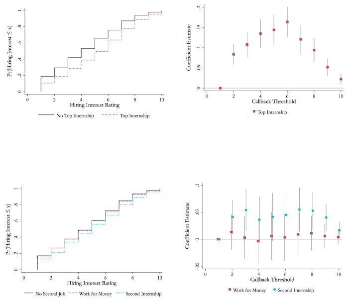
Figure 1: Value of Quality of Experien ce Over Selectivity Distribution
(a) Empirical CDF for Top Internship
(b) Linear Probability Model for Top In-
ternship
(c) Empirical CDF for Second Job Type
(d) Linear Probability Model for Second
Job Type
Empirical CDF of Hiring Interest (Panels 1a & 1c) and di↵erence in counterfactual callback rates
(Panels 1b & 1d) for Top Internship, in the top row, and Second Internship and Work for Money,in
the bottom row. Empirical CDFs show the share of hypothetical candidate resumes with each char-
acteristic with a Hiring Interest rating less than or equal to each value. The counterfactual callb a ck
plot shows the di↵erence between group s in the s h a re of candidates at or above the threshold—that
is, the share of candidates who would be cal led back in a resume audit stud y if the callback thresh-
old were set to any given value. 95% confidence intervals are calculated from a linear probability
model with an indicator for being at or above a threshold as the dependent variable.
23
While we see no evidence of discrimination on average, a large literature address-
ing diversity in the sciences (e.g., Carrell et al. [2010], Goldin [2014]) suggests we
might be particularl y likely to see d is cr i mi nat i on among employers seeking STEM
candidates. In Table 3, we estimate the regression in Equation (1) separately by
major type. Results in Columns 5-10 show that employers looking for STEM can-
didates display a large, statistically significant prefer en ce for white male candidates
over white females and non-white males. The coefficients on Female, W hi te and
Male, Non-W hi te suggest that these candidates su↵er a pen al ty of 0.5 Likert-scale
points—or about 0.27 GPA poi nts—that is robust across our specifications. These
e↵ects are at least marginally significant even after multiplying our p-values by two
to correc t for the fact t hat we are analyzing our results within two subgroups (uncor-
rected p-values are: p =0.009 for Female, White; p =0.049 for Male, Non-White).
Results in Columns 1-5 show no evidence of discrimination in hiring interest among
Humanities & Social Sciences employers.
As in Section 3.3, we can examin e t h es e r es ul t s across the hiring interest rating
distribution. Figure 2 shows the CDF of hiring interest ratings and the di↵erence in
counterfactual callback rates. For ease of interpretation and for statistical power, we
pool female and minority candidates and compare them to white male candidates
in these figures and in some analyses that follow. The top row shows these compar-
isons for employers interested in Humanities & Social Sci e nc es candidates and the
bottom row shows these compari son s for employers interested in STEM candidates.
Among employers interested in Humanities & Social Sciences candidates, the CDFs
of Hiring I nterest ratings are nearly identical. Among employers interested in STEM
candidates, however, the CDF for white male candidates first order st ochastically
dominates the CDF for cand id at es who are not white males. At the point of the
largest counterfactual callback gap, employers i nterested in STEM candidates would
display callback rates that were 10 percentage points lower for candidates who were
not white males than for thei r white male counterparts.
One might be surprised that we find any evidence of discrimination, given that
employers may have (correctly) believed we would not use demographic tastes in
generating t h ei r matches and given that employers may have attempted to override
any discriminatory preferen ce s to be more socially acceptable. One possibility for
why we nevertheless find discr im in at ion is the role of implicit bias [Greenwald et al.,
1998, Nosek et al., 2007], which Bertrand et al. [2005] has suggested is an important
24

channel f or discrimination in resume audit studies. In Appen d ix B.4, we explore
the role of implicit bias in driving our results.
24
In particular, we leverage a feature
of implicit bias—that it is more likely to arise when de ci si on makers are fatigued
[Wigboldus et al., 2004, Govorun and Payne, 2006, Sherman et al., 2004]—to test
whether our data are consistent with employers displaying an implicit racial or
gender bias. As shown in Appendix Table B.7, employers spend less time evaluating
resumes both in the latter half of the study and in the latter half of each set of 10
resumes (after each set of 10 resumes, we introduced a short break for subjects),
suggesting evidence of fatigue. Discrimination is statistically significantly larger
in the latter half of each block of 10 resumes, providing suggestive evidence that
implicit bias plays a role in our findings, although discrimination is not larger in the
latter half of the study.
Race and gender could also subconsciously a↵ect how employers view other re -
sume components. We test for negative interactions between race and gender and
desirable candidate characteristics, which have been found in the resume audit lit-
erature (e.g., minority status has been shown to lower returns to resume quali ty
[Bertrand and Mullainathan, 2004]). Appendix Table B.8 i nteracts Top Intern-
ship, our binary variable most predictive of hiring interest, with our demographic
variables. These interactions are all direct i on al ly negative, and t h e coefficient Top
Internship ⇥ Female, White is negative and significant, suggesting a lower ret u r n
to a prestigious internships for white females. One possible mechanism for this ef-
fect is t h at employers believe that other employers exhib i t positive preferences for
diversity, and so having a prestigious internship is a less strong signal of quality
if one is from an under-represented group. This aligns with the findings shown in
Appendix Figure B.6, which shows that the negative interaction between Top In-
ternship and demographics appears for candidates with r el at i vely low ratings and is
a fairly precisely estimated zero when candidates receive relatively high ratings.
24
Explicit bias might include an explicit taste for whi t e male c a n d id a t es or a n explicit belief they
are more prepared than female or minority candidates for success at their firm, even conditional on
their resumes. Implicit bias [Greenwald et al., 1998, Nosek et al., 2007], on the other hand, may
be present even among employers who are not expli ci t ly considering race (or among employers who
are considering race but attempting to suppress any explicit bias they might have).
25

Table 3: E↵ects by Major Type
Dependent Variable: Hiring Interest
Humanities & Social Sciences STEM
OLS OLS OLS
GPA-Scal e d
OLS
Ordered
Probit OLS OLS OLS
GPA-Scal e d
OLS
Ordered
Probit
GPA 2.208 2.304 2.296 1 0.933 1.932 1.885 1.882 1 0.802
(0.173) (0.179) (0.153) (.) (0.0735) (0.267) (0.309) (0.242) (.) (0.112)
Top Internship 1.075 1.043 1.033 0. 450 0.452 0.398 0.559 0.545 0.289 0.175
(0.108) (0.116) (0.0945) (0.0500) (0.0461) (0.191) (0.216) (0.173) (0.0997) (0.0784)
Second Internship 0.540 0.516 0.513 0.224 0.240 0.242 0.307 0.311 0.165 0.111
(0.132) (0.143) (0.114) (0.0514) (0.0555) (0.208) (0.246) (0.189) (0.103) (0.0881)
Work for Money 0.0874 0.107 0.116 0.0504 0.0371 0.151 0.275 0.337 0.179 0.0761
(0.129) (0.134) (0.110) (0.0477) (0.0555) (0.212) (0.254) (0.187) (0.102) (0.0881)
Technical Skills 0.0627 0.0841 -0.0502 -0.0219 0.0132 -0.0283 -0.113 -0.180 -0.0959 -0.000579
(0.122) (0.130) (0.106) (0.0463) (0.0522) (0.197) (0.228) (0.186) (0.0998) (0.0831)
Female, White -0.0466 -0.117 -0.0545 -0.0237 -0.0154 -0.419 -0.612 -0.545 -0.290 -0.171
(0.134) (0.142) (0.117) (0.0510) (0.0566) (0.215) (0.249) (0.208) (0.115) (0.0895)
Male, Non-White -0.0293 -0.0100 -0.0259 -0.0113 -0.00691 -0.567 -0.617 -0.507 -0.270 -0.265
(0.158) (0.169) (0.137) (0.0595) (0.0664) (0.271) (0.318) (0.257) (0.136) (0.111)
Female, Non-White 0.0852 0.101 0.0909 0.0396 0.0245 -0.329 -0.260 -0.0465 -0.0247 -0.142
(0.160) (0.171) (0.137) (0.0599) (0.0680) (0.264) (0.301) (0.261) (0.138) (0.111)
Observations 2040 2040 2040 2040 2040 840 840 840 840 840
R
2
0.128 0.196 0.500 0.119 0.323 0.593
p-value for test of joi nt
significance of Majors 0.021 0.027 0.007 0.007 0.030 < 0.001 0.035 < 0.001 < 0.001 < 0.001
Major FEs Yes Yes Yes Yes Yes Yes Yes Yes Yes Yes
Leadership FEs No Yes Ye s Yes No No Yes Yes Yes No
Order FEs No Yes Yes Yes No No Yes Yes Yes No
Subject FEs No No Yes Yes No No No Yes Yes No
Ordered probit cutpoints (Column 5): 2.25, 2.58, 2.96, 3. 2 6, 3.60, 3.94, 4.41, 4.86, 5.41.
Ordered probit cutpoints (Column 10): 1.44, 1.90, 2.22, 2 . 51 , 2.80, 3.14, 3.56, 4.05, 4.48.
Table shows OLS and ordered probit reg ress io n s of Hiring Interest from Equation (1). Robust stand a rd errors are reported in parentheses. GPA; Top Internship ;
Second Internship; Work for Money; Technical Skil ls ; Female, White ; Male, Non-White; Female, Non-White and major are characteristics of the hypothetic a l
resume, constructed as described in Sect io n 2.3 and in Appendix A.2. Fixe d e↵ects for major, leadershi p experience, resume ord er, and subject included as indicated.
R
2
is indicated for each OLS regression. GPA-Scaled OLS presents the results of Column 3 and Column 8 divided by the Column 3 and Co lu m n 8 coefficients on
GPA, w it h standard errors calc u la t ed by delta method . The p-values of tests of joint significance of major fi xe d e↵ects are indicat ed (F -test for OLS, likelihood ratio
test for ordered probit) after a Bonferroni correction for analyzing two subgroups.
26
3.5 Candidate Likelihood of Accept ance
In resume audit stud i es, traits that suggest high candidate q ual i ty do not always
increase employer callback. For example, several studies have found that employers
call back employed candidates at lower rates than unemployed candid at es [Kroft
et al., 2013, Nunley et al., 2017, 2014, Farber et al., 2018], but that longer peri-
ods of unemployment are unappealing to employers. This seeming contradiction
is consistent with the hypothesis that employers are concerned about the possi-
bility of wasting resources pursuing a candidate who will ultimate ly reject a job
o↵er. In other words, hiring interest is not the only factor determining callback
decisions. This concern has been acknowledged in the resume audi t literature, for
example when Bertrand and Mullainathan [2004, p. 992] notes, “In creating the
higher-quality res um es , we deliberately make small changes in credentials so as to
minimize the risk of overqualification.”
As d es cr i bed in Section 2.4, for each resume we asked employers “How likely do
you think [Name] would be to accept a job with your organization ?” Ask i n g th is
question helps ensure that our measure of hiring interest is unconfounded with con-
cerns that a candidate would accept a position when o↵ered. However, the q u est i on
also allows us to study this second factor, which also a↵ects callback decisi on s.
Table 4 replicates the regression spe ci fi cat i ons from Table 2, estimating Equation
(1)whenV
ij
is Likelihood of Acceptance, which takes values from 1 to 10. Employers
in our sample view high quality candidates as more likely to accept a job with their
firm t han low quality candidates. Thi s suggests that employers in our sample believe
candidate fit at their firm outweighs the possibility that high quality candidates will
be pursue d by many other firms. In Appendix B.5, we further consider the role of
horizontal fit and vertical quality and find that—holdi ng hiring interest in a candi-
date constant—reported likelihood of acce pt an ce falls as evidence of vertical quality
(e.g., GPA) increases. This r esu l t highlights that there is independent information
in the likelihood of acceptance measure.
Table 4 s hows that employers report female and minority candidates are less
likely to accept a position with their firm, by 0.2 points on the 1–10 Likert scale
(or about one tenth of a standard deviation). This e↵ect is robust to the inclusion
of a variety of controls, and i t persists when we hold hiring interest constant in
Appendix Table B.9. Table 5 splits the sample and shows that while the direction
27
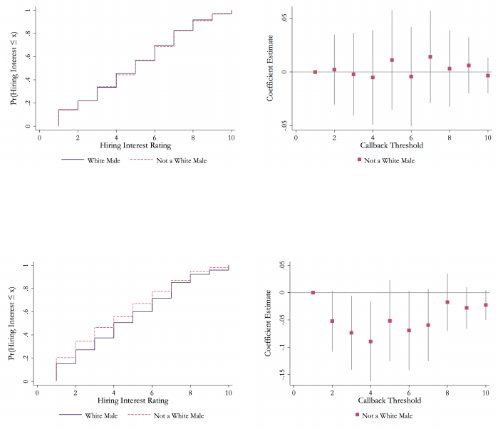
Figure 2: Demographics by Major Type Over Selectivity Distribution
(a) Empirical CDF: Not a White Male, Hu-
manities & Social Sciences
(b) Linear Probabi l i ty Model: Not a White
Male, Humanities & Social Sciences
(c) Empirical CDF: Not a White Male,
STEM
(d) Linear Probabi l i ty Model: Not a White
Male, STEM
Empirical CDF of Hiring Interest (Panels 2a & 2c) and di↵erence in counterfactual callback rates
(Panels 2b & 2d) for White Male and Not a White Male. Employers interested in Humanities &
Soc ia l Sciences candidates are shown in the top row and employers interested in STEM candidates
are shown in the bottom row. Empirical CDFs show the share of hypothetical candidate resumes
with each characteristic with a Hiring Interest rating less than or equal to each value. The coun-
terfactual callback plot shows the di↵erenc e between groups in the share of candidates at or above
the threshold—that is, the share of candidates who would be called back in a resume audit study
if t h e callback threshold were set to any given val u e. 95% confidence intervals are calculated from
a linear probability model with an indicator for being at or above a threshold a s the dependent
variable.
28

of these e↵ects is consistent among both groups of employers, the negative e↵ects
are particularly large among employers recruiting STEM candidates.
If minority and female applicants are perceived as less likely to accept an o↵er,
this could induce lower callback rates for these candidates. Our results therefore
suggest a new channel for discrimination observed in the labor market, which is
worth exploring. Perhaps due to the prevalence of diversity initiatives, employers
expect that desirable minority and female candidates will receive many o↵ers from
competing firms and thus will be less l i kely to accept any given o↵er. Alternatively,
employers may see female and minority candi d at es as less likely to fit in the culture
of the firm, making these candidates less likely to accept an o↵ er . This r es ul t has
implications for how we understand the labor market and how we interpret the
discrimination observed in resume audit studies.
25
3.6 Comparing our Demographic Results to Previous Literature
3.6.1 Qualitative comparison
Our results can be compar ed to those from other studies of employer preferences,
with two caveats . First, our measure of the fir ms ’ interest in hiring a candidate may
not be directly comparable to findings derived from callback rates, which likely com-
bine both hiring interest and likelihood of acceptance into a sin gl e binary outcome.
Second, our subject p op ulat i on is made up of firms that would be unlikely to re-
spond to cold resumes and thus may h ave di↵erent preferences than the typical firms
audited in prior literature.
Resume audit studies have consistently shown lower callback rates for minori-
ties. We see no evidence of lower ratings for minorities on average, but we do see
lower ratings of minority male cand id at es by STEM employers. Results on gen-
der in the resume audit literature have been mixed. In summarizing results from
11 studies conducted between 2005 and 2016, [Baert, 2018] finds four studies wit h
higher callback rates for women, two with lower callback rates, and five studies
with no significant di↵erence. None of these studies found discrimination against
25
In particular, while audit studies can demonstrate that groups are not being treat ed equally,
di↵erential c a llb a ck rates need not imply a la ck of employer interest. The impact of candidate
characteristics on likelihood of acceptance is a case of omitted variable bias, but one that is not
solved by experimental randomization, since th e ra n d o mi ze d t rai t en d ows the candidate with hiring
interest and likelihood of acceptance simultaneously.
29

Table 4: Likelihood of Acceptance
Dependent Variable: Likelihood of Accept anc e
OLS OLS OLS
Ordered
Probit
GPA 0.605 0.631 0.734 0.263
(0.144) (0.150) (0.120) (0.0603)
Top Internship 0.683 0.677 0.664 0.285
(0.0943) (0.0979) (0.0763) (0.0396)
Second Internship 0.418 0.403 0.394 0.179
(0.112) (0.119) (0.0911) (0.0472)
Work for Money 0.197 0.192 0.204 0.0880
(0.111) (0.116) (0.0896) (0.0467)
Technical Skills -0.0508 -0.0594 -0.103 -0.0248
(0.104) (0.108) (0.0861) (0.0435)
Female, White -0.231 -0.294 -0.258 -0.0928
(0.114) (0.118) (0.0935) (0.0476)
Male, Non-White -0.125 -0.170 -0.117 -0.0602
(0.137) (0.142) (0.110) (0.0574)
Female, Non-White -0.221 -0.236 -0.162 -0.103
(0.135) (0.142) (0.112) (0.0568)
Observations 2880 2880 2880 2880
R
2
0.070 0.124 0.492
p-value for test of joi nt
significance of Majors < 0.001 < 0.001 < 0.001 < 0.001
Major FEs Yes Yes Yes Yes
Leadership FEs No Yes Yes No
Order FEs No Yes Yes No
Subjec t FEs No No Yes No
Ordered probit cutpoints: -0.26, 0.13, 0.49, 0.75, 1.12, 1.49, 1.94, 2.46, and 2 .8 3 .
Table shows OLS and ordered probit regressions of Likelihood of Accep-
tance from Equation (1). Robust standard errors are reported in parenthe-
ses. GPA; Top Internship; Second Internship; Work for Money; Technical
Skills; Female, White; Male, Non-White; Female, Non-White and major are
characteristics of the hypothetical resume, constructed as described in Sec-
tion 2.3 and in Appendix A.2. Fixed e↵ects for major , leadership experience,
resume order, and subject included in some specifications as indicated. R
2
is
indicated for each OLS regression. The p-values of tests of joint significance
of major fixed e↵ects are indicated (F -test for OLS, l i kelihood ratio test f or
ordered probit).
30

Table 5: Likelihood of Acceptance by Major Type
Dependent Variable: Likelihood of Accept anc e
Humanities & Social Sciences STEM
OLS OLS OLS
Ordered
Probit OLS OLS OLS
Ordered
Probit
GPA 0.581 0.610 0.694 0.251 0.688 0.724 0. 813 0.314
(0.176) (0.186) (0.142) (0.0719) (0.251) (0.287) (0.237) (0.110)
Top Internship 0.786 0.773 0.754 0.316 0.391 0.548 0. 527 0.190
(0.111) (0.118) (0.0892) (0.0458) (0.178) (0.199) (0.171) (0.0782)
Second Internship 0.481 0.422 0.424 0.201 0.254 0.324 0.301 0. 119
(0.136) (0.148) (0.109) (0.0553) (0.198) (0.230) (0.187) (0.0880)
Work for Money 0.206 0.173 0.187 0.0845 0.155 0.346 0.350 0.0923
(0.135) (0.144) (0.108) (0.0553) (0.194) (0.239) (0.186) (0.0878)
Technical Skills -0.0942 -0.103 -0.106 -0.0460 0.0495 0.000154 -0.116 0.0316
(0.125) (0.134) (0.104) (0.0521) (0.190) (0.217) (0.179) (0.0830)
Female, White -0.175 -0.211 -0.170 -0.0615 -0.365 -0.572 -0.577 -0.177
(0.139) (0.148) (0.116) (0.0564) (0.198) (0.236) (0.194) (0.0892)
Male, Non-White -0.0691 -0.0756 -0.0462 -0. 0296 -0.269 -0.360 -0.289 -0.147
(0.161) (0.172) (0.130) (0.0662) (0.259) (0.302) (0.246) (0.110)
Female, Non-White -0.244 -0.212 -0.163 -0.107 -0.200 -0.108 -0.0103 -0.105
(0.162) (0.175) (0.130) (0.0679) (0.243) (0.278) (0.245) (0.110)
Observations 2040 2040 2040 2040 840 840 840 840
R
2
0.040 0.107 0.516 0.090 0.295 0.540
p-value for test of joi nt
significance of Majors 0.798 0.939 0.785 0.598 < 0.001 0.001 < 0.001 < 0.001
Major FEs Yes Yes Yes Yes Yes Yes Yes Yes
Leadership FEs No Yes Ye s No No Yes Yes No
Order FEs No Yes Yes No No Yes Yes No
Subjec t FEs No No Yes No No No Yes No
Ordered probit cutpoints (Column 4): -0.23, 0.14, 0.50, 0 .7 5 , 1.11, 1.48, 1.93, 2.42, 2.75.
Ordered probit cutpoints (Column 8): -0.23, 0.20, 0.55, 0 .8 3 , 1.25, 1.64, 2.08, 2.71, 3.57.
Table shows OLS and ordered probit regressions of Likelihood of Acceptance from Equation (1). GPA; Top Internship ; Second
Internship; Work for Money; Technical Skil ls ; Female, White ; Male, Non-White; Female, Non-White and major are characteristics
of the hypothet ic a l resume, constructed as described in S e ct i on 2.3 and in Appendix A.2. Fixed e↵ects for major, leadership
experi enc e, resume order, and subject included as indicated. R
2
is indicated for each OLS regression. Th e p-values of tests of
joint significance of major fixed e↵ects are indicated (F -test for OLS, likelihoo d ratio test for ordered pro b it ) after a Bonferroni
correction for analyzing two su b g ro u p s.
31

women in a U.S. setting. This may be due to resume audit studi es targeting female-
dominated occupations, such as clerical or administrative work. Riach and Rich
[2006], which specifically targets male-dominated occupations, shows lower call back
rates for women. Outside t he labor market, Bohren et al. [2018] and Milkman et al.
[2012] found evidence of discrimination against women using audit-type meth od-
ology. We find that firms recruiting STEM candidates give lower ratings to white
women, demonstrating the importance of being able to reach new subject pools with
IRR. We also find that white women r ec ei ve a lower return to prestigious intern-
ships. This result matches a type of discrimination—lower return to quality—seen
in Bertrand and Mullainathan [2004], but we find it for gender rather than race.
We also find that empl oyers believe white women are less likely to accept posi-
tions if o↵ered, which coul d account for discrimination found in the resume audit
literature. For example, Quadlin [2018] finds t h at women with very high GPAs are
called back at lower rates than women with lower GPAs, which could potentially
arise from a belief these high quality women will be recruited by other fir ms , rather
than from a lack of hiring interest.
3.6.2 Quantitative comparison using GPA as a nu me rai re
In addition to making qualitati ve comparisons, we can conduct some back-of-
the-envelope calculations to compare the magnitude of our demographic e↵ects to
those in previous studies, including Bertrand and Mullainathan [2004]. We conduct
these comparisons by taking advantage of the ability—in our study and others—to
use GPA as a numeraire.
In studies that randomize GPA, we can di v i de the observed e↵ect due to race or
gender by the e↵ect due to GPA to compare with our GPA-scale d estimates. For
example, exploiting th e random variation in GPA and gender from Quadlin [2018],
we calculate that being female leads t o a decrease in callback equivalent to 0.23 GPA
points.
26
Our results (sh own in Tables 2 and 3) suggest that being a white female,
26
Quadlin [2018] reports callback rate in four GPA bins. The paper finds callback is lower in the
highest GPA bin than the second highest bin, which may be due to concerns about likelihood of
acceptance. Looking at the second and third highest bins (avoiding the non-monotonic bin), we see
that an increase in GPA from the range [2.84, 3.20] to [3.21, 3.59]—an average increase of 0.38 G PA
poi nts—results in a call b a ck rate increase of 3.5 percentage points. Dividing 0.38 by 3.5 su g g es ts
that each 0.11 GPA points generates 1 percentage point di↵erence in callback rates. Quadlin [2018]
also finds a callback di↵erence of 2.1 percentage points between male (14.0%) and female (11.9%)
candidates. Thus, applicant gender has about the same e↵ect as a 0.23 change in GPA.
32

as compared to a white male, is equival ent to a d ec re ase of 0.073 GPA points overall
and 0.290 GPA points among employers recruiting for STE M .
When a study does not vary GPA, we can benchmark the e↵ect of demographic
di↵erences on callback to the e↵ect of GPA on counterfactual callback in our study.
For example, in Bertrand and Mullainathan [2004], 8% of all resumes receive call-
backs, and having a black name decreases callback by 3.2 percentage points. 7.95%
of resume s in our study receive a 9 or a 10 rating, suggesting that receiving a 9 or
higher is a similar level of selectivity as in Bertr and and Mullainathan [2004]. A
linear probability model in our data s ugge st s that each 0.1 GPA point increases coun-
terfactual callback at this threshold by 1.13 percentage points. Thus, the Bertrand
and Mullainathan [2004] race e↵ect is equivalent to an increase of 0.28 GPA points
in our stud y.
27
This e↵ect can be compared to our estimate that being a minori ty
male, as compared to a white male, is equivalent to a decrease of 0.077 GPA points
overall and 0.270 GPA points among employers recruiting for STEM.
4 Pitt Replicatio n: Results and Lessons
In order to explore whether preferences di↵ered between employers at Penn (an
elite, Ivy League school) and other institutions where recruiters might more closely
resemble the employers of typical resume audit studies, we reached out to several
Pennsylvania schools in hopes of running an IRR replication. We partnered with the
University of Pittsburgh (Pitt) Office of Career Development and Placement Assis-
tance to run two experimental rounds during thei r spring recruiting cycle.
28
Ideally,
27
Bertrand and Mullainathan [2004] also varies quality, but through changing multiple charac-
teristics at once. Using the same method, these changes, which alter callb a ck by 2.29 percentage
poi nts, are equivalent t o a change of 0.20 GPA points, providing a benchmark for th eir quality
measure is in our GPA points.
28
Unlike at Penn, there is no major fall recruiting season with elite firms at Pitt. We recruited
employers in the spring semester on l y, first in 2017 and again in 2018. The Pitt recru i tm ent
email was similar to that used at Penn (Figure A.1), and originated from the Pitt Office of Career
Development and Placement Assistance. For the first wave at Pitt we o↵ered webinars, as described
in Appendix A.1,butsinceattendanceatthesesessionswaslow,wedidnoto↵ertheminthesecond
wave. We collected resume components to populate the tool at Pitt from real resumes of graduating
Pitt seniors. Rathe r than collect resumes from clubs, resume books, and campus job postings as
we did at Penn, we used the candidate pool of j ob- se eki n g seniors both to populate the tool and
to suggest matches for employers. This significantly eased the burden of collecting and scraping
resumes. At Pitt, majors were linked to either the “Dietrich School of Art s and Sciences” or the
“Swanson School o f Engineering”. Table C.1 lists the majors, associated school, major category,
and the probability that the major was drawn. We collected top internships at Pitt by identifying
33

the comparison between Penn and Pitt would have given us additional insight into
the extent to which Penn emp loyers di↵ered from employers traditionally target e d
by audit studi e s.
Instead, we learned that we were insufficiently attuned t o how recruiting di↵er-
ences between Penn and Pitt employer populations should influence IRR implemen-
tation. Specifically, we observed significant attenuation over nearly all candidate
characteristics in the Pitt data. Table 6 shows fully controlled OLS regressions
highlighting that our e↵e ct s at Pitt (shown in the secon d column) are directionally
consistent with those at Penn (shown in the first column for reference), but much
smaller in size. For example, the coefficient on GPA is one-tenth the size in the
Pitt data. We find similar attenuation on nearly all characteristics at Pitt for both
Hiring Interest and Likelihood of Acceptance, in the pooled sample and separated
by major type. We find no evidence of Pitt employers responding to candidate de-
mographics. (Appendix C provides details for our experimental implementation at
Pitt and Tables C.2, C.3, and C.4 display the full results.)
We suspect the cause of the attenuation at Pitt was our failure to appropriately
tailor resumes to meet the needs of Pitt employers who were seeking can d id at es
with specialized skills or backgrounds. A large share of the resumes at Pitt ( 33. 8%)
received the lowest possible Hiring Interest rating, more than double the share at
Penn (15.5.%). Feedback from Pitt employers suggested that they were also less
happy with their matches: many respondents complained that the m at ches lacked
a p art ic ul ar skill or major req u ir e ment for their open positions.
29
In addition,
the importance of a maj or requirement was reflected on the post-su r vey data in
which 33.7% of Pitt employers indicated that candidate major was among the most
important considerations dur i n g recruitment, compared to only 15.3% at Penn.
After observing these issues in the first wave of Pitt data collection, we added a
new checklist question to t he post-tool survey in t h e second wave: “I would consider
candidates for this position with any of the following majors.. . .” This question
allowed us both to restrict the match pool for each employer, improving match
quality, and to directly assess the extent t o which ou r failure to t ai l or resumes was
the firms hiring the most Pi tt graduates, as at Penn. Top internships at Pitt tended to be less
prestigious th a n the top internships at Penn.
29
As one example, a firm wrote to us in an email: “We are a Civil Engineering firm, specifically
focu s ed on hiring students out o f Civil and/or Environmental Engineering programs... there are 0
students in the group of rea l resumes that you sent over that are Civil Engineering students.”
34
attenuating our estimates of candidate characteristics. Table 6 shows that when
splitting the d ata from the second wave based on whet he r a candidate was in a
target major, the e↵ect of GPA is much larger in the target major sample (shown
in the fourth column), and that employers do not respond strongly to any of the
variables when considering candidates with majors that are not Target Majors.
The di↵erential responses depending on whether resumes c ome from Target Ma-
jors highlights the importance of tailoring candidate resumes to employers when
deploying the IRR methodology. We advertised the survey tool at both Pitt and
Penn as being particularly valuab l e for hiring skilled generalists, and we were ill
equipped to measure preferences of employers looking for candidates with very par-
ticular qualifications.
This was a limitation in our implementation at Pitt rather than in the IRR
methodology itself. That is, one could design an IRR study specifical l y for employ-
ers interested in hiring registered nurses, or employers interested in hiring mobile
software developers, or employers interested in h i ri n g electrical engineers. Our fail-
ure at Pitt was in showing all of these employers resumes wi t h the same underlying
components. We recommend that researchers using IRR either target employers
that specifically recruit high quality generalists, or construct resumes with appr o-
priate variation within the employers’ targe t areas. For example, if we ran our IRR
study again at Pitt, we would ask the Target Majors q u es ti on first an d then only
generate hypothetical resumes from t hos e majors.
5 Conclusion
This paper introduces a novel methodology, called Incentivized Resume Rating
(IRR), to measure employer preferences . The method has employers rate candidate
profiles they know to be hypoth et i cal and provides incentives by matching employers
to real job seekers based on their reported preferences.
We deploy IRR to study employer preferences for candidates graduating from an
Ivy League university. We find that employers highly value both more p r est i gi ou s
work experience the summer bef or e senior year and additional work experience the
summer before junior year. We use our ten-point rating data to demonstr ate that
preferences for these characteristics are relatively stable throughout the distribu t i on
of candidate quality. We find no evidence that employers are less interested in
35

Table 6: Hiring Interest at Penn and Pitt
Dependent Variable: Hiring Interest
Penn Pitt
Pitt, Wave 2
Non-Target Major
Pitt, Wave 2
Target Major
GPA 2.196 0.265 -0.196 0.938
(0.129) (0.113) (0.240) (0.268)
Top Internship 0.897 0.222 0.0199 0.0977
(0.0806) (0.0741) (0.142) (0.205)
Second Internship 0.466 0.212 0.0947 0.509
(0.0947) (0.0845) (0.165) (0.220)
Work for Money 0.154 0.153 0.144 0.378
(0.0914) (0.0807) (0.164) (0.210)
Technical Skills -0.0711 0.107 0.125 -0.0354
(0.0899) (0.0768) (0.149) (0.211)
Female, White -0.161 0.0279 -0.0152 -0.151
(0.0963) (0.0836) (0.180) (0.212)
Male, Non-White -0.169 -0.0403 0.00154 -0.331
(0.115) (0.0982) (0.185) (0.251)
Female, Non-White 0.0281 -0.000197 0.182 -0.332
(0.120) (0.100) (0.197) (0.256)
Observations 2880 3440 642 798
R
2
0.483 0.586 0.793 0.596
p-value for test of joi nt
significance of Majors < 0.001 < 0.001 0.120 0.850
Major FEs Yes Yes Yes Yes
Leadership FEs Yes Yes Yes Yes
Order FEs Yes Yes Yes Yes
Subject FEs Yes Yes Yes Yes
Table shows OLS regressions of hiring interest from Equation (1). Sample di↵ers in
each column as indicated by the column header. Robust standard errors are reported
in parentheses. GPA; Top Internship; Second Internship; Work for M oney; Technical
Skills; Female, White; Male, Non-White; Female, Non-White and major are charac-
teristics of the hyp ot he t ic al resume, constr uc te d as described in Section 2.3 and in
Appendix A.2. Fixe d e↵ects for major , leadership experience, resume order, and sub-
ject included in all specifications. R
2
is indicated for each OLS regressi on . The p-value
of an F -test of joint significance of m ajor fixed e↵ects is indicated for all models.
36

female or min ority candidates on average, but we find evidence of discrimination
among employers recruiting STEM candidates. Moreover, employers report that
white female candidates are less likely to accept job o↵ers than their white male
counterparts, a novel channel for discrimination.
Here, we further di s cu ss the benefits and costs of the IRR methodology, high-
light lessons learned from our impl em entation—which point to improvements in the
method—and discuss directions for future research.
A key advantage of the IRR methodology is that it avoids the use of deception.
We speculate t h at economics has tolerated the use of deception in correspondence
audit studies in part because of the absence of a deception-free alternative. We
developed IRR to provide such an alternative. The availability of an alternative is
particularly important given the recent proliferation of decept i ve audit studies both
within labor economics and into settings beyond labor markets. As discussed in the
Introduction, the increasing use of audit studies within labor markets risks contam-
inating the subject pool—biasi n g estimates from future audit studies and harming
real applicants whose profiles look like fake candidates created by rese archers.
Extending deception in new settings may have add i t ion al unintended conse-
quences. As prominent examples, researchers have recently audited college pro-
fessors requesting in-person meetings [Milkman et al., 2012, 2015] and politicians
requesting information [Butler and Broockman, 2011, Distelhorst and Hou, 2017].
Professors ar e likely to learn ab ou t audit studies ex post and may take the existence
of such studies as an excuse to ignore emails from students in the future. Audits
of politicians’ respon ses to correspondence from putative constituents might distor t
politicians’ beliefs about the priorities of the populations they serve, especially when
researchers seek a politician-level au dit measure, which requires sending many fake
requests to the same politician.
We hope that further development of the IRR method w il l lead to stricter stan-
dards for when deception can be u sed in economics research and that it will be a
welcome change even among researchers who run audit studies, since reducing the
number of decept ive audit studies limits contamination of the subject pool.
A second advantage of the IRR method is that it elicits richer preference infor-
mation than binary callback decisions.
30
In our implementation, we elicit granular
30
Bertrand and Duflo [2016] argues that the literature has generally not evolved past measuring
di↵erences in callback means between groups, and that it has been less successful in illuminat in g
37

measures of employers’ hiring interest and of employers’ beliefs about the likelihood
of job acceptance. We also see the potential for improvements in preference elicita-
tion by better mapping t he se metrics into hiring dec i si ons , by collecting additional
information from employers, and by rais in g the stakes, which we discuss below.
The IRR method has other advantages. IRR can access subje ct populations
that are inaccessible with audit or resume audit methods. IRR al l ows researchers to
gather rich data from a single subject—each employer in our implementation rates
40 resumes—which is helpful for power and makes it feasible to identify preferences
for characteristics within individual subjects. IRR allows researchers to random-
ize many candidate characteristics independently and simultaneously, which can be
used to explore how employers respond to interactions of candidate characteristics.
Finally, IRR allows resear chers to collect supplemental data about research sub-
jects, which can be cor re l at ed with subject-level preference measures and allows
researchers to better unde r st and their pool of employers .
A final advantage of IRR is that it may provide direct benefits to subjects and
other participants in the labor market being st u di ed ; this advantage stands in stark
contrast to using subject time without consent, as is necessary in audit studies.
We solicited subject feedback at numerous points throughout the study and heard
very few concern s.
31
Instead, many employers re ported positive feedback. Positive
feedback also came by way of the career services offices at Penn and Pitt, which
were in more direct contact wi t h our employer s ubjects. Both offices continued
the experiment for a second wave of recruit me nt and expressed interest in making
the experiment a permanent feature of their recruiting process. In our meetings,
the career services offices reported seeing value in IRR to improve their matching
process and to le ar n how employers valued student characteristics (thus informing
the advice they could give to students ab ou t pursuing summer work and leadership
mechanisms driving these di↵erences. That said, there have been some exceptions, like Bartoˇs et al.
[2016], which uses emails containing l in k s to lea rn mo re about candidates to show that less atten-
tion is allo ca t ed to can d id at es who are discriminated against. Another exception is Bohren et al.
[2018], which uses evaluations of a n swers posted on an online Q&A forum—which are not conflated
with concerns about likelihood of acceptance—to test a dynamic model of mista ken discriminatory
beliefs.
31
First, we solicited feedback in an o pen comments field of the survey itself. Second, we invited
participants to contact us with question s or requests for additional matches when we sent the
10 resumes. Third, we ran a follow-up survey in which we asked about hiring outcomes for the
recommended matches (unfortuna t ely, we o↵ered n o incentive to complete the follow-up survey and
so its participation was low).
38

experience and how to write their resumes). While we did not solicit feedback from
student participants in t h e study, we received hundreds of resumes f rom students at
each school, suggesting that they valued the prospect of having their resumes sent
to employers.
32
Naturally, IRR also has some limitations. Because the IRR method informs
subje ct s that responses will be used in research, it may lead to experimenter demand
e↵ects (see, e.g., de Quidt et al. [2018]). We believe the impact of any experimenter
demand e↵ects is likely small, as employers appeared to view our survey tool as a
way to identify promising candidates, rather than as being connect ed to research
(see discussion in Section 2). For this reason, as well as others highlighted in Section
3.4, IRR may be less well equipped to identify explicit bias than implicit bias. More
broadly, we cannot guarantee that employers treat our hypothetical resumes as they
would real job can di d at es. As discussed in the Introduction, however, future work
could help validate emp l oyer attention in IRR studies.
33
In addition, because the
two outcome measures in our study are hypothetical objects rather than stages of the
hiring process , in our implementation of IRR we cannot draw a direct link between
our findings and hiring outc omes . Below, we discuss how this might be improved in
future IRR implementations.
Finally, running an IRR stu dy requi re s finding an appropriate subject pool and
candidate matching pool, which may not be available to all researchers. It also
requires an investment in constructing the hypothetical resumes (e.g., scraping and
sanitizing resume components) and developing the process to match employer pref-
erences to candidates. Fortunately, the time and resources we devoted to developing
the survey tool software can be leveraged by other researchers.
Futu re research using IRR can certainly improve upon our implementation.
First, as discussed at length in Section 4, our failed attempt to r ep l i cat e at Pitt
highlights that future re sear chers must take care to e↵ectively tailor the content
32
Student involvement only re qu ire d uploading a resume a n d completing a short preference survey.
We did not notify students when they were matched with a firm, in order to give the firms freedom
to choose which students to contact. Thus, most students were u n aware of whether or not they
were recommended to a firm. We recommended 207 unique student resumes over the course of the
study, highlighting the value to students.
33
The time employers spent evaluating resumes in our study at Penn had a median of 18 seconds
and a mean that was substantially higher (and varies based on how outliers are handled). These
measures are comparable to estimates of time spent screening real resumes (which include estimates
of 7.4 secon d s per resume [Dishman, 2018] and a mean of 45 seconds per resume [Culwell-Block
and Sellers, 1994]).
39

of resumes to match the hiring needs of their subjects. Second, we suggest de-
veloping a way to tran sl at e Likert-scale responses to the callback deci si on s typical
in correspondence audit studies. One idea is to ask employers to additionally an-
swer, p ot e ntially for a subset of resumes, a question of the form: “Would you invite
[Candidate Name] for an interview?” By having the Likert-scale responses and
this measure, r es ear chers could identify what combination of the hiring interest and
likelihood of acceptance responses translates into a typical callback decision (and,
potentially, how the weight placed on each component varies by firm). Researchers
could also explore the origin and accuracy of employer belie fs about likelihood of
acceptance by asking job candidates about their willingness to work at participat-
ing firms. Thi r d, researchers could increase the stakes of IRR incentives (e.g., by
asking employer subjects to guarantee interviews to a subset of the recommended
candidates) an d gather more information on interviews and hiring outcomes (e.g.,
by building or leveraging an existing platform to measure employer and candidate
interactions).
34
While we used IRR to measure the preferences of employers in a particular labor
market, the underlying incentive structure of the IRR method is much more general,
and we see the possibility of it being applied outside of the resume rating context.
At the heart of IRR is a method to elicit preference infor mat i on from experimen-
tal subject s by having them evaluate hypothetical objects and o↵ering them an
incentive that increases in value as preference reports become more accurate. Our
implementation of IRR achieves this by eliciting continuous Likert-scale measures
of hypothetical resumes, using machine learning to esti mat e the extent to which
employers care about various candidate characteristics, and providing employers
with resumes of real candidates that they are estimated to like best. Researchers
could take a similar strate gy to expl or e pref er en ce s of profess ors over prospective
students, landlords over tenants, customers over products, individuals over dating
profiles, and more, providing a powerful antidote to the growth of deceptive studies
in economics.
34
An additional benefit of collecting data on interviews and hiring is that it would allow re-
searchers to bett er validate the val u e of matches to employers (e.g., researchers could identify 12
pot ential matches and randomize which 10 are sent to employers, identifying the e↵ect of sending
a resume t o employers on interview and hiring outcomes). If employers do respond to the matches,
one could imagin e using IRR as an intervention in labor markets to help mitigate discrimination in
hiring, since IRR matches can be made while ig n o rin g race and gender.
40
References
Joseph G Altonji and Rebecca M Blank. Race and gender in the labor market.
Handbook of Labor Economics, 3:3143–3259, 1999.
David H Autor and Susan N Houseman . Do temporary-help jobs improve labor
market outcomes for low-skilled workers? Evidence fr om “Work First”. American
Econom ic Journal: Applied Economics , pages 96–128, 2010.
Stijn Baert. Chapter 3: Hiring discrimination: An overview of (almost) all corre-
spondence experiments since 2005. In Michael S. Gaddis, editor, Audit Studies:
Behind the Scenes with Theory, Method, and Nuance, chapter 3, pages 63–77.
Springer, 2018.
Vojtˇech Bartoˇs, Michal Bauer, Julie Chytilov´a, and Filip Matˇejka. Attention dis-
crimination: Theory and field experiments with monitoring information acquisi-
tion. American Economic Review, 106(6):1437–75, June 2016. doi: 10.1257/aer.
20140571.
Marianne Bertrand and Esther Duflo. Field experiments on discrimination. NBER
Worki ng Papers 22014, National Bureau of Economic Research, Inc, Feb 2016.
Marianne Bertrand and Se nd hi l Mullai nat h an. Are Emily and Gr eg more employable
than Lakisha and Jamal? The American Economic Review, 94(4):991–1013, 2004.
Marianne Bertrand, Dolly Chugh, and Sendhil Mullainathan. Implicit discrimina-
tion. American Economic Review, 95(2):94–98, 2005.
Iris Bohnet, Alexandra Van Geen, and Max Bazerman. When performance trumps
gender bias: Joint vs. separate evaluation. Management Science, 62(5):1225–1234,
2015.
J. Aislin n Bohren, Alex Imas, and Michael Rosenberg. The dynamics of discrimi-
nation: Theory and evidence. American Economic Review (Forthcoming), 2018.
Daniel M. Butler and David E. Broockman. Do politicians racially discriminate
against constituents? A field ex periment on state legislators. American Journal
of Political Science, 55(3):463–477, 2011.
41
Scott E. Carrel l , Marianne E. Page, and James E. West. Sex and science: How pro-
fessor gender perpetuates the gender gap. The Quarterly Journ al of Economics,
125(3):1101–1144, 2010.
Beverly Culwell-Block and J ean Anna Sellers. Resume con-
tent and format - do the authorities agree?, Dec 1994. URL
https://www.questia.com/library/journal/1G1-16572126/
resume-content-and-format-do-the-authorities-agree.
Rajeev Darolia, Cory Koedel, Paco Martorell, Katie Wilson, and Francisco Perez-
Arce. Do employers prefer worker s who attend for-profit col l ege s? Eviden ce from
afieldexperiment. Journal of Policy Analysis and Management, 34(4):881–903,
2015.
Jonathan de Quidt, Johannes Haushofer, and Chr is t oph er Rot h. Measuring and
bounding exper i menter demand. American Economic Review, 108(11) : 3266–3302,
November 2018. doi: 10.1257/aer.20171330. URL http://www.aeaweb.org/
articles?id=10.1257/aer.20171330.
David J. Deming, Noam Yuchtman, Amira Abulafi, Claudia Goldin, and
Lawrence F. K at z. The value of postsecondary credentials in the labor mar -
ket: An experimental study. American Economic Review, 106(3):778–806, March
2016.
Lydia Dishman. Your resume only gets 7.4 seconds to make an impression–here’s
how to stand out, Nov 2018. UR L https://www.fastcompany.com/90263970/
your-resume-only-gets-7-4-seconds-to-make-an-impression-heres-how-to-stand-out.
Greg Distel hor st and Yue Hou. Constituenc y service under nondemocratic rule:
Evidence from China. The Journal of Politics, 79(3):1024–1040, 2017. doi: 10.
1086/690948.
Stefan Eriksson and Dan-Olof Rooth. Do employers use u ne mp loyment as a sorting
criterion when hiring? Evidence from a field experiment. American Economic
Review, 104(3):1014–39, March 2014. d oi : 10.1257/aer.104.3.1014.
Michael Ewens, Bryan Tomlin, and Liang Choon Wang. Statistical discrimination or
prejudice? A large s amp le field experiment. Review of Economics and Statistics,
96(1):119–134, 2014.
42
Henry S Farber, Chris M Herbst, Dan Silverman, and Till von Wachter. Whom do
employers want? The role of recent employment and unemployment status and
age. Working Paper 24605, National Bureau of E con omi c Research, May 2018.
Roland G. Fryer and Steven D. Levitt. The causes and consequences of distinctively
black names. Q uar ter l y Journal of Economics, 119:767–805, 2004.
S. Michael Gaddis. Discr im i nat i on in the credential society: An audit study of race
and college selectivity in the labor market. Social Forces, 93(4):1451–1479, 2015.
Claudia Goldin. A grand gender convergence: Its last chapter. American Economic
Review, 104(4):1091–1119, 04 2014.
Olesya Govorun and B Keith Payne. Ego–depletion and prejudice: Separating au-
tomatic and controlled components. Social Cognition, 24(2):111–136, 2006.
William Greene. The behaviour of the maximum likelihood estimator of limited
dependent variable models in t h e presence of fixed e↵ects . The Econometrics
Journal, 7(1):98–119, 2004.
Anthony G Greenwald, Debbi e E McGhee, and Jordan LK Schwartz. Measuring
individual di↵erences in implicit cognition: the implicit association test. Journal
of personali ty and social psychology, 74(6):1464, 1998.
Daniel Hamermesh. Are fake resumes ethical for academic research? Freakonomics
Blog, 2012.
Andrew Hanson and Zackary Hawley. Do landlords discriminate in the rental housing
market? Evidenc e from an internet field experiment in US cities. Journal of Urban
Econom ics , 70(2-3):99–114, 2011.
Glenn W. Harrison and John A. List. Field experi m ents. Journal of Economic
Literature, 42(4):1009–1055, December 2004. doi: 10.1257/0022051043004577.
James J. Heckman. D e t ect i n g discrim in at i on. Journal of Economic Perspectives, 12
(2):101–116, 1998.
James J. Heckman and Peter Siegelman. The Urban Institute audit studies: their
methods and findings. In Clear and convincing evidence: measurement of discrim-
ination in America, pages 187–258. Lanhan, MD: Urban Institute Press, 1992.
43
Lars J Kirkeboen, Edwin Leuven, and Magne Mogstad. Field of study, earnings,
and self-selection. The Quarterly Journal of Economics, 131( 3) : 1057–1111, 2016.
Meredith Kleykamp. A great place to start?: The e↵ect of prior mil i t ary ser-
vice on hiring. Armed Forces & Society, 35(2):266–285, 2009. doi: 10.1177/
0095327X07308631.
Kory Kroft, Fabian Lange, and Matthew J. Notowidigdo. Duration dependence
and labor market conditions: Evidence from a field experiment. T he Quarterly
Journal of Economics, 128(3):1123–1167, 2013. doi: 10.1093/qje/qjt015.
Kevin Lang and Jee-Yeon K Lehmann. Racial discrimination in the labor market:
Theory and empirics. Journal of Economic Literature, 50( 4) : 959–1006, 2012.
Corinne Low. A “reproductive capital” model of marriage market matching.
Manuscript, Wharton School of Business, 2017.
Katherine L. Milkman, Modupe Akinola, and Dolly Chugh. Temporal distance and
discrimination: an audit study in academia. Psychological Science, 23(7):710–717,
2012.
Katherine L. Milkman, Modupe Akinola, and Dolly Chugh. What happens before?
A field experiment exploring how pay and representation di↵erentially shape bias
on the pathway into organizations. Journal of Applied Psychology, 100(6), 2015.
David Neumark. Detecting discrimination in audit and correspondence studies.
Journal of Human Resources, 47(4):1128–1157, 2012.
David Neumark, Ian Burn, and Patrick Button. Is it harder for older workers to
find jobs? New and improved evidence from a field experiment. Technical report,
National Bureau of Economic Research, 2015.
Brian A Nosek, Frederick L Smyth, Je↵rey J Hansen, Thierry Devos, Nicole M
Lindner, Kate A Ranganath, Colin Tucker Smith, Kristina R Olson, Dolly Chugh,
Anthony G Greenwald, et al. Pervasiveness an d correlates of implicit attitudes
and stereotypes. European Review of Social Psychology, 18(1):36–88, 2007.
John M Nunley, Adam Pugh, Nicholas Romero, and R Alan Seals. Unemployment,
underemployment, and employment opportunities: Results from a correspondence
44
audit of the labor market for college graduates . Auburn University Department
of Economics Working Paper Series, 4, 2014.
John M. Nunley, Adam Pugh, Nicholas Romero, and R. Alan Seals. The e↵ects of
unemployment and underemployment on employment opportunities: Results from
a correspondence audit of the labor market for college graduates. ILR Review, 70
(3):642–669, 2017.
Andreas Ortmann and Ralph Hertwig. The costs of deception: Evidence from
psychology. Experimental Economics, 5(2):111–131, 2002.
Amanda Pallais. Inefficient hiri ng in entry-level labor markets. American Economic
Review, 104(11):3565–99, 2014.
Devin G Pope and Justin R Sydnor. What’s in a picture? Evidence of discrimination
from prosper.com. Journal of Human resources, 46(1):53–92, 2011.
Natasha Quadlin. The mark of a woman’s record: Gender and academic performance
in hiring. American Sociological Review, 83(2):331–360, 2018. doi: 10.1177/
0003122418762291. URL https://doi.org/10.1177/0003122418762291.
Peter A Riach and Judith Rich. An experimental investigation of sexual discrimi-
nation in hir i ng in the English labor market. Advances in Economic Analysis &
Policy, 5(2), 2006.
Lauren A. Rivera and Andr´as Tilcsik. Class advantage, commitment penalty: T he
gendered e↵ect of social class signals in an elite labor market. American Soci-
ologi cal Review, 81(6):1097–1131, 2016. doi: 10.1177/0003122416668154. URL
https://doi.org/10.1177/0003122416668154.
Je↵rey M Rzeszotarski, Ed Chi, Praveen Paritosh, and Peng Dai. Inserting micro-
breaks into crowdsourcing workflows. In First AAAI Conference on Human Com-
putation and Crowdsourcing, 2013.
Je↵rey W Sherman, Frederica R Conrey, and Carla J Groom. Encoding flexibili ty
revisited: Evidence for enhanced encoding of stereotype-inconsistent information
under cognitive load. Social Cognition, 22(2):214–232, 2004.
45
Margery Turner, Michael Fix, and Raymond J. Struyk. Opportunities denied, op-
portunities, diminished : racial discrimination in hiring. Washington, DC: Urban
Institute Press, 1991.
Dani¨el HJ Wigboldus, Je↵rey W Sherman, Heather L Franze se, and Ad van Knip-
penberg. Capacity and comprehension: Spontaneous stereotyping under cognitive
load. Social C ognition, 22(3):292–309, 2004.
Asaf Zussman. Ethnic disc ri m in at i on: Lessons f r om the Israeli online market for
used cars. The Economic Journal, 123(572):F433–F468, 2013.
46
FOR ONLINE PUBLICATION ONLY
Appendices
We provide three appendices. In Appendix A, we describe the design of our
experiment in detail, i n cl u din g recruit ment materials (A.1), survey tool construc-
tion (A.2), and the candidate matching process (A.3). In Appendix B,wepresent
additional analyses and results, includin g human capital results (B.1), regressions
weighted by GPA (B.2), a discussion of our discrimination results (B.4), and a dis-
cussion of preferences over the quality distribution (B.3). In Appendix C,wediscuss
additional details related to repl i cat i n g our experiment at Pitt.
A Experimental Design Appendix
A.1 Recruitment Materials
University of Pennsylvania Career Services sent recruitment materials to both
recruiting firms and grad u ati n g seniors to participate in the study. All materials
marketed the st u dy as an additional tool to connect students with firms, rather than
a replacement for any usual recr ui t i ng e↵orts. The recruitment email for employers,
shown in Fi gu re A.1, was sent to a list of contacts maintained by Career S er v i ces and
promised to use a “newly developed machine-learning algorithm to identify candi-
dates who would be a particularly good fit for your job based on your evaluations.”
In our repli c at ion at the University of Pittsburgh, a similar email was sent from the
Pitt Office of Career Development and Placement Assistance.
Penn Career Services r ec r ui t ed graduating seniors to participate as part of the
candidate matching pool through their regular newsletter called the “Friday Flash.”
The relevant excerpt from this email newsletter is shown in Figure A.2.
We timed recruitment so that employe rs would receive their 10 resume matches
around the tim e they were on campus in order to facilitate meeting the job seek-
ers. In addition, we o↵ered webinars for employers who were interested in learning
about the survey screening experience before t he y participated. Employers could
anonymously join a call wher e they viewed a slideshow about the survey software
and could submit questions via chat box. Attendance at these webinars was low.
47
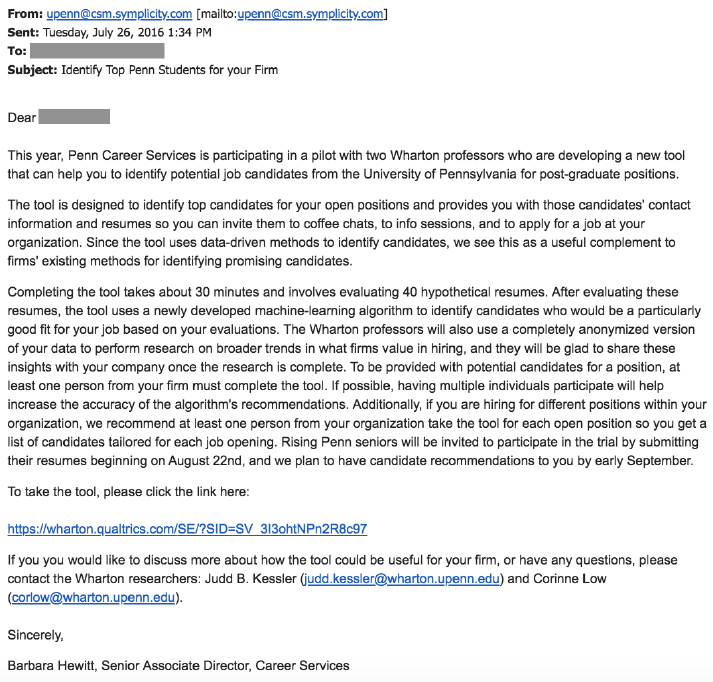
Figure A.1: Employer Recruitment Emai l
Email sent to firms recruiting at Penn origin a t i n g fro m th e S en io r As sociate Director of Career
Services at the University of Pennsylvania. Subjects who followed the link in the email were taken
to the instructions (Figure A.3).
48
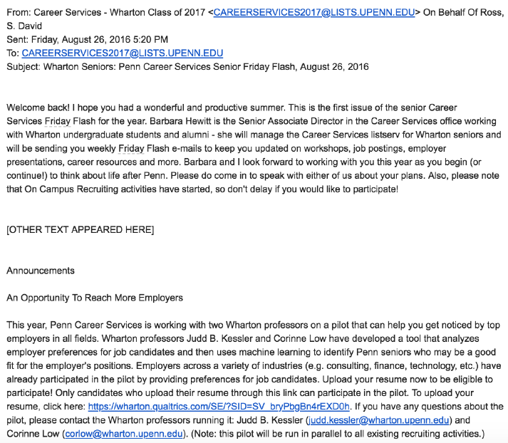
Figure A.2: Email Announcement to Graduating Seniors
Excerpt from email newsletter sent to the Career Services office m a il in g list. The email originated
from the Sen io r Associate Director of Career Services at the University of Pennsylva n ia . Students
following the link were taken to a survey page where they were asked to upload their resumes and
to answer a brief questionnaire about their job se arch (pag e not shown).
49
A.2 Survey Tool Design
In this appendix, we describe the process of generating hypotheti cal resumes.
This appendix should serve to provide additional details ab out the selection and
randomization of resume components, and as a guide to researchers wishing to i m-
plement our methodology. In S ec t ion A.2.1, we describe the structur e of the IRR
survey t ool and participant experi e nc e. In Section A.2.2,wedescribethestructure
of our hypothetical resumes. In Section A.2.3, we detail the randomization of can-
didate gender and race through names. Section A.2.4 det ai ls the randomization of
educational background. Section A.2.5 describes the process we used to collect and
scrape real resume components to randomize work experience, leadership experience,
and skills.
A.2.1 Survey Tool Structure
We constructed the survey tool us in g Qualtrics software for respondents to access
from a web browser. Upon opening the s ur vey link, respondents must enter an
email address on the instructions page (see Figure A.3) to continue. Respondents
then sele ct the type of candidates they will evaluate for their open p osi t i on, either
“Business (Wharton), Social Sciences, and Humanities” or “Science, Engineering,
Computer Science, and Math.” In addition, they may enter the pos i ti on title they
are looking to fill. The position title is not used in determining the content of
the hypotheti cal candidate resumes. The major selection page is shown i n Figure
A.4. After this selection, the randomization software populates 40 resumes for the
respondent to evaluate, drawing on di↵erent content by major type. T he subject
then evaluates 40 hypothetical resumes. After every 10 resumes, a bre ak page
encourages subjects to continue.
A.2.2 Resume Structure
We designed our resumes to combine realism wit h the requirements of experi-
mental identification. We designed 10 resume templates to use as the basis for the
40 resumes in the tool. Each template presented the same information, i n the same
order, but with variations in page layout and font. Figur e s A.5 and A.6 show sam-
ple resume templates. All resumes contained five sections, in the foll owing order:
Personal Information (incl ud i ng name and blurred contact information); Education
50

Figure A.3: Survey Tool Instructions & Contact Information
Screenshot of the inst ru c ti o n s at the start of the survey tool. This page provided information to
subjects and served as instructions. Subjects entered an email a d d res s at the bottom of the screen
to proceed with the study; the resumes of the 10 real job seekers used as an incentive to participate
are sent to this email address .
51
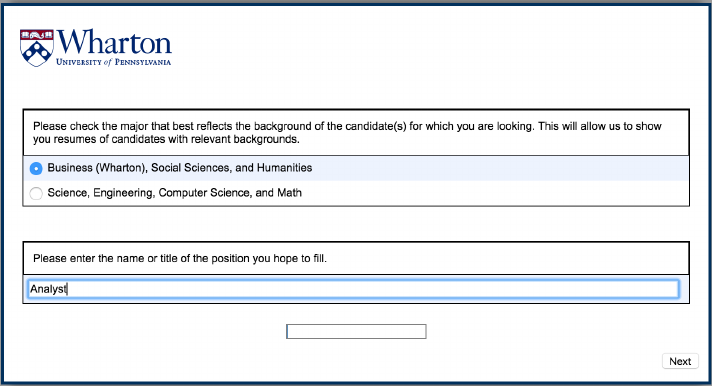
Figure A.4: Major Type Selection
Screenshot of major selection page, as shown to subjects recruiting at t h e University of Pennsylva-
nia. Subjects must select either Business (Wharton), Social Sciences, and Humanities, or Scie n ce ,
Engineering, Computer Science, and Math. Subjects may also enter th e name of the positio n they
wish to fill in the free text box; the informa t io n in this box was not used for analysis. Here, we
have selected Business (Wharton), Social Sciences, and Humanities and entered “Analyst” as a
demonstration only—by default all radio boxes and t ext boxes were empty for all subjects.
52

(GPA, major, school within uni versity); Work Experience; Leadership Experience;
and Skills.
35
While the real student resumes we encountered varied in content,
most contained some subset of these sections. Since our main objective with resume
variation was t o imp r ove realism for each subject rather than to test the e↵ective-
ness of di↵erent resume formats, we did not vary the order of the resume formats
across subjects. In other words, the first resume always had the same font and
page layout for each subject, although the content of the resume di↵ered each time.
Given that formats are in a fixed order in the 40 hypothetical resumes, the order
fixed e↵ects included in most specifications control for any e↵ect of resume format.
Resumes templates were built in HTML/CSS f or display in a web browser, and pop-
ulated dynamically in Qualtrics using JavaScript. Randomization occurred for all
40 resumes simultaneously, without replacement, each time a subject completed the
instructions an d selected their major category of interest. Each resume layou t was
flexible enough to accommodate di↵erent numbers of bullet points for each experi-
ence, and di↵erent numbers of work experiences. If on ly one job was listed on the
resume, for instance, the work experience section of the resume appeared shorter
rather than introducing empty space.
35
These sections were not always labelled as such on candidate resumes. Personal Information
was generally not identified, though each resume contained a name and blurred text in place of
contact information. Skills were also marked as “Skills & Interests” and “Skill Summary”.
53
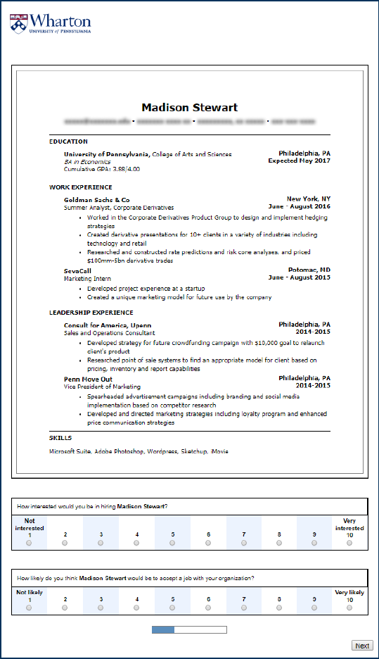
Figure A.5: Sample Resume
A sample resume rating page from the Incentivized Resume Rating tool. Each resume is dynamically
generated when the subject begins the study. Each resume has five sections: Personal Information (including
first and last name, and blurred text to represent contact information); Educ a t io n Information (university,
school within un iversity, degree, major, GPA, and expected graduation date); Work Experience (one or
two experiences with employer name, location, job title, date, an d descriptive bullet p o i nts); Leadership
Experi enc e (two exp erie n ce s with organization, location, position title, date, and descriptive bullet points);
and Skills. Resume randomization described in detail in Section 2 and Appendix A.2.Atthebottomof
each resume, subjects must respond t o two questions before proceeding: “How interested would you be in
hiring [Name]?” and “How likely do you think [Name] would be to accept a job with your organization?”
54
A.2.3 Names
A hypothetical candidate name ap pears as the fi rs t element on each re su me.
Names were generated to be highly indicative of race and gender, following the
approach of Fryer and Levitt [2004]. As described in Section 2.3.4, first names were
selected from a dataset of all births in the state of Massachusetts between 1989-
1996 and in New York City between 1990-1996. These years reflect the appr oximate
birth years of the job seekers in our stud y. We identified 100 first names with the
most indic at ive race and ge nd er for each of the following race-gender combinations:
Asian Female, Asian Male, Black Female, Black Male, Hispanic Female, Hispanic
Male, White Female, and White Male. We then eliminated names that were gender-
ambiguous in the broad sample even if they might be unambiguous within an ethnic
group. We also eliminated names strongly indicative of religion. We followed a
similar process for last names, using name and ethn i ci ty data from the 2000 Census.
Finally, we paire d first and last names together by race and selected 50 names
for each race-gender combination for randomizat i on. Names of hypothetical female
candidates are shown i n Table A.1; names of hypothetical male candidates are shown
in Table A.2.
At the point of randomization, names were drawn without replacement accord-
ing to a distribution of race and gender intended to reflect the US population (50%
female, 50% male; 65.7% White, 16.8% Hispanic, 12.6% Black, 4.9% Asian). Gender
and race were randomiz ed independently. In other words, we selected either Table
A.1 or Table A.2 with equal probability, then selected a column to draw from accord-
ing to the race probabilities. Final l y, names were selected uniformly and without
replacement from the appropri at e column of the table. We use the variat i on induced
by these names for the analysis variables Female, White; Male, Non-White; Female,
Non-White; and Not a White Male.
55
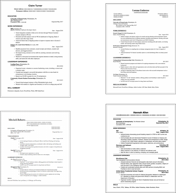
Figure A.6: Four Sample Resumes
Four sample resumes generated by the survey to o l. Note that the resum es each have a di↵erent
format, di↵erentiated by elem ents such as font, boldface type, horizontal rules, location of informa-
tion, and spacing. All resumes have the same five sections: Personal Information, Education, Work
Experi enc e, Leadership Experience, and Skills. Resumes di↵er in length based on the dynamically
selected content, such as the randomized number of work experiences and the (non-randomized)
number of description bullet points associated wit h an experience.
56

Table A.1: Female Names Populating Resume Tool
Asian Female Black Female Hispanic Female White Female
Tina Zheng Jamila Washington Ivette Barajas Allyson Wood
Annie Xiong Asia Je↵erson Nathalie Orozco Rachael Sullivan
Julie Xu Essence Banks Mayra Zavala Katharine Myers
Michelle Zhao Monique Jackson Lui s a Vel azq ue z Colleen Peterson
Linda Zhang Tianna Joseph Jessen ia Meza Meghan Miller
Anita Zhu Janay Mack Darlene Juarez Meaghan Murphy
Alice Jiang Nia Williams Thalia Ibarra Lindsey Fisher
Esther Zhou Latoya Robinson Perla Cervantes Paige Cox
Winnie Thao Jalisa Coleman Lissette Huerta Katelyn Cook
Susan Huang Imani Harris Daisy Espinoza Jillian Long
Sharon Yang Malika Sims Cristal Vazquez Moll y Baker
Gloria Hwang Keisha James Paola Cisneros Heather Nelson
Diane Ngo Shanell Thomas Leticia Gonzalez Alison Hughes
Carmen Huynh Janae D i x on Je sen i a Hernandez Bridget Kel l y
Angela Truong Latisha Daniels Alejandra Contreras Hayley Russell
Janet Kwon Zakiya Franklin Iliana Ramirez Carly Roberts
Janice Luong Kiana Jones Julissa Esparza Bethany Phil li p s
Irene Cheung Ayana Grant Giselle Alvarado Kerry Bennett
Amy Choi Ayanna Holmes Gloria Macias Kara Morgan
Shirley Yu Shaquan a Frazier Selena Zuniga Kaitlyn Ward
Kristine Nguyen Shaniqua Green Maribel Ayala Audrey Rogers
Cindy Wu Tamika Jenkins Liliana Mejia Jacquelyn Mar t in
Joyce Vu Akilah Fields Arlene Rojas Marissa Anderson
Vivian Hsu Sh antel Simmons Cristina Ochoa Haley Clark
Jane Liang Shanique Carter Yaritza Carillo Lindsay Campbell
Maggie Tsai Tiara Woods Guadalupe Rios Cara Adams
Diana Pham Tierra Bryant Angie Jimenez Jenna Morris
Wendy Li Raven Brown Esmeralda Maldonado Caitlin Price
Sally Hoang Octavia Byrd Marisol Cardenas Kathryn Hall
Kathy Duong Tyra Walker Denisse Chavez Emma Bailey
Lily Vang Diamond Lewis Gabriela Mendez Erin Collins
Helen Trinh Nyasia Johnson Jeanette Rosales Marisa Reed
Sandy Oh Aliyah Dougl as Rosa C ast ane da Madeleine Smith
Christine Tran Aaliyah Alexander Beatriz Rodriguez Mackenzie King
Judy Luu Princess Henderson Yessenia Acevedo Sophie Thompson
Grace Cho Shanae Richardson Carolina Guzman Madison Stewart
Nancy Liu Kenya Brooks Carmen Agu i lar Margaret Parker
Lisa Cheng Charisma Scott Yesenia Vasq u ez Kristin Gray
Connie Yi Shante Hunter Ana Munoz Michaela Evans
Ti↵any Phan Jada Hawkins Xiomara Ortiz Jaclyn Cooper
Karen Lu Shanice Reid Lizbeth Rivas Hannah Allen
Tracy Chen Chanelle Sanders Genesis Sosa Zoe Wilson
Betty Dinh Shanequa Bell St e ph any Salinas Caitlyn Young
Anna Hu Shaniece Mitchell Lorena Gutierrez Charlotte Moore
Elaine Le Ebony Ford Emely Sandoval Kaitlin Wright
Sophia Ly Tanisha Watkins Iris Villarreal Holly White
Jenny Vo Shanelle Butler Mari t za Garza Kate Taylor
Monica Lin Precious Davis Marilyn Arroyo Krista Hill
Joanne Yoon Asha Willis Lou rd es Soto Meredith Howard
Priya Patel Ashanti Edwards Gladys Herrera Claire Turner
Names of hypothetical female candidates. 50 names were selected to be highly indicative of each combination
of race and gender. A name drawn from these lists was displayed at the top of each hypothetical resume, and
in the questions used to evaluate the resumes. First and last names were linked every time they appe a red .
For details on the construction and randomizatio n of names, see Section 2.3.4 and Appendix A.2.3.
57

Table A.2: Male Names Populating Resume Tool
Asian Male Black Male Hispanic Male White Male
Richard Thao Rashawn Washington Andres Barajas Kyle Wood
Samuel Truong Devonte Je↵erson Julio Oroz co Derek Sullivan
Daniel Cheung Marquis Banks Marcos Zavala Con nor Myers
Alan Tsai Tyree Jackson Mike Velazquez Douglas Peterson
Paul Li Lamont Joseph Jose Meza Spencer Miller
Steven Zhang Jaleel Mack Alfredo Juarez Jackson Murphy
Matthew Zheng J avon Williams Fern an do Ibarra Bradley Fisher
Alex Vu Darryl Robinson G us t avo Cervantes Drew Cox
Joshua Vo Kareem Coleman Adonis Huerta Lucas Cook
Brandon Lu Kwame Harris Juan Espin oza Evan Long
Henry Dinh Deshawn Sims Jorge Vazque z Adam Baker
Philip Hsu Terrell James Abel Cisneros Harris on Nelson
Eric Liang Akeem Thomas Cesar Gonzalez Brendan Hughes
David Yoon Daquan Dixon Alberto Hernandez Cody Kelly
Jonathan Yu Tarik Daniels Elvin Contreras Zachary Russell
Andrew Trinh Jaquan Franklin Ruben Ramirez Mitchell Roberts
Stephen Yi Tyrell Jones Reynaldo Esparza Tyler Phillips
Ryan Nguyen Isiah Grant W il f r ed o Alvarado Matthew Bennett
Aaron Jiang Omari Holmes Francisco Macias Thomas Morgan
Kenneth Zhao Rashad Frazier Emi li o Zuniga Sean War d
Johnny Hwang Jermai ne Green Javier Ayala Nicholas Rogers
Tony Choi Donte Jenkin s Guillermo Mejia Brett Martin
Benjamin Luong Donnell Fields Elvis Rojas Cory Anderson
Raymond Tran Davon Simmons Miguel Ochoa Colin Clark
Michael Duong Darnell Carter Sergio Carillo Jack Campbell
Andy Hoang Hakeem Woods Alejandro Rios Ross Adams
Alexander Pham Sheldon Bryant Ernesto Jimenez Liam Morris
Rob er t Yang Antoine Brown Oscar Maldonado Max Price
Danny Xu Marquise Byrd Felix Cardenas Ethan Hall
Anthony Huynh Tyrone Walker Manuel Chavez Eli Bailey
Jason Liu Dashawn Lew is Orlando Mendez Pat r i ck Collins
John Chen Shamel Johns on Luis Rosales Luke Reed
Brian Vang Reginald Douglas Eduard o Castaneda Alec Smith
Joseph Zhou Shaquille Alexand er Carlos Rodriguez Seth King
James Cho Jamel Henders on Cristian Acevedo Austin Thompson
Nicholas Lin Akil Richardson Pedro Guzman Nathan Stewart
Je↵rey Huang Tyquan Bro ok s Freddy Aguilar Jacob Parker
Christopher Wu Jamal Scott Esteban Vasquez Craig Gray
Timothy Ly Jabari Hunter Leonardo Munoz Garrett Evans
William Oh Tyshawn Hawkins Arturo Ortiz Ian Cooper
Patrick Ngo Demetrius Reid Jesus Rivas Benjamin Alle n
Thomas Cheng Denzel Sanders Ramon Sosa Conor Wilson
Vincent Le Tyreek Bell Enrique Salinas J are d You n g
Kevin Hu Darius Mitchell Hector Gutierrez Theodore Moore
Jimmy Xiong Prince Ford Armando Sandoval Shane Wright
Justin Zhu Lamar Watkins Roberto Villarreal Scott White
Calvin Luu Raheem Butler Edgar Garza Noah Taylor
Edward Kwon Jamar Davis Pablo Arroyo Ryan Hill
Peter Phan Tariq Willis Raul Soto Jake Howard
Victor Patel Shaquan Edwards Diego Herrera Maxwell Turner
Names of hypothetica l male candidates. 50 names were selected to be highly indicative of each combination
of race and gender. A name drawn from these lists was displayed at the top of each hypothetical resume, and
in the questions used to evaluate the resumes. First and last names were linked every time they appe a red .
For details on the construction and randomizatio n of names, see Section 2.3.4 and Appendix A.2.3.
58
A.2.4 Education
We randomized two components in the Education section of each resume: grade
point average (GPA) and major. We also provided an exp ec te d graduation date
(fixed to M ay 2017 for all students), t he name of the university (University of Penn-
sylvania), the degree (BA or BS) and the name of the d egr ee- granting school within
Penn to maintain realism.
GPA We selected GPA from a Unif[2.90, 4.00] distributi on , rounding to the near-
est hundredth. We chose to include GPA on all resumes, although some students
omit GPA on real resumes. We decided to avoid the complexity of forcing subjects
to make inferences about missing GPAs . The range was selected to approximate the
range of GPAs observed on real resumes. We chose a uniform distribu t ion (rather
than, say, a Gaussi an ) to increase our power to identify preference s throughout
the distribution. We did not specify GPA in major on any resumes. We use this
variation to define the variable GPA.
Major Majors for the hypothetical resumes were selected accordin g to a predefined
probability distrib ut i on intended t o balance the realism of the rating experience and
our ability to detect and control for the e↵ect of majors. Table A.3 shows e ach major
along with its school affi l iat i on and classification as Humanities & Social Sciences
or STEM, as well as the probability assigned to each. We use this variation as th e
variable Major and control for it with fixed e↵ects in most regression s.
A.2.5 Components from Re al Resumes
For work exp er i en ces , leadership experiences, and skil ls , we drew on components
of resumes of real Penn students. This design choice improved the realism of the
study by matching the tone and content of real Penn job see kers. Moreover, it
improved the validity of our results by ensuring that our distribution of resume
characteristics is close to the true distribution. This also helps us identify the range
of interest for the study, since resumes of unrealistically low (or high) quality are
unlikely to produce usef ul variation f or identification.
Source resumes came from campus database s (for example, student club resume
books) and from seniors who submitted their resumes in order to participate in the
59

Table A.3: Majors in Generated Penn Res um es
Type School Major Probability
Humanities &
Social Sciences
The Wharton School BS in Economics 0.4
College of Arts and Sci en ce s
BA in Economics 0.2
BA in Political Science 0.075
BA in Psychology 0.075
BA in Communication 0.05
BA in English 0.05
BA in History 0.05
BA in History of Art 0.025
BA in Philosophy 0.025
BA in International Relations 0.025
BA in Sociology 0.025
STEM
School of Engineering and
Applied Science
BS in Computer Engineering 0.15
BS in Biomedical Science 0.075
BS in Mechanical Engineering and Applied Mechanics 0.075
BS in Bioengineering 0.05
BS in Chemical and Bi omol ec ul ar Engineering 0.05
BS in Cognitive Science 0.05
BS in Computational Biology 0.05
BS in Computer Science 0.05
BS in Electrical Engineering 0.05
BS in Materials Science and Engineering 0.05
BS in Networked and Social Systems Engineering 0.025
BS in Systems Science and Engineering 0.025
College of Arts and Sci en ce s
BA in Biochemistry 0.05
BA in Biology 0.05
BA in Chemistry 0.05
BA in Cognitive Science 0.05
BA in Mathematics 0.05
BA in Physics 0.05
Majors, degrees, schools within Penn, and th e ir selection probability by major type. Majors (and
their associated degrees and schools) were drawn with replacement and randomized to resumes
after subjects s elec t ed to view either Humanities & Social Sciences resumes or STEM resumes.
60
matching process. When submitting resumes, students were informed that com-
ponents of their resumes could be shown di r ec tl y to employers. We scrape d these
resumes using a commerci al resume parser (the Sovren Parser). From the scraped
data we compiled one list with collections of skills, and a second list of experi-
ences comprising an organization or employer, a position title, a loc ati on , and a job
description (generally in the for m of resume bullet points).
Resume components were selected to be interchangeable across resumes. To that
end, we cleaned each work experience, leadership experience, and skills lis t in the
following ways:
• Re moved any infor mat i on that might indicate gender, race, or religion (e.g.,
“Penn Women’s Varsi ty Fencing Team” was changed to “Penn Varsity Fencing
Team” and “Penn Muslim Stu de nts Association” was not used)
• S cr ee ne d out components indicative of a specific major (e.g., “Explorat or y
Biochemistry Intern” was not used)
• Cor r ec te d grammatical errors
Work Experience We designed our resumes to vary both the quality and quan-
tity of work experience. All resumes had a work experien ce during the summer
before the candidate’s senior year (June–August 2017). This work experience was
either a regular internship (20/40) or a top internship (20/40). In addition, some
resumes also had a second work experience (26/40), which varied in quality between
a work-for-money job (13/40) or a regular internship (13/40). The job title, em-
ployer, description, and location shown on the hypothetical resumes were the same
as in the source resume, with the minimal cleaning described above.
Before selecting the work experiences, we defi ne d a Top Internship to be a sub-
stantive position at a pre st i gi ous employer. We chose this definition to both identify
prestigious firms and distinguish between di↵erent types of jobs at those firms, such
as a barista at a local St ar bu cks and a marketing intern at Starbucks headquar-
ters. We identified a prestigious employer to b e one of the 50 firms hiring the most
Penn grad uat es in 2014 ( as compiled by our Career Serv ic es partners). S i nc e experi-
ences at these firms were much more comm on among Humanities & Social Sciences
majors, we supplemented this list with 39 additional firms hir i ng most often from
Penn’s Scho ol of Engineering and Applied Science. We ext r act e d experiences at
61

these firm s from our full list of scraped experiences, and selec t ed a total of 40 Top
Internship experiences, with 20 coming from resumes of Humanities & Social Sci-
ences majors and 20 from resumes of STEM majors. All of these Top Internship
experiences had to be believably interchangeable within a major category. These
internships in cl u de d positi ons at Bain Capital, Goldman Sachs, Morgan Stanley,
Northrop Grumman, Boeing Company, and Google (see Table A.4 for a complete
list). This variation identified the variable Top Internship in our analysis, which is
measured relative to having a regular internship (since all r esu me s had some job in
this position).
Table A.4: Top Internship Employers
Humanities &
Social Scien ces STEM
Accenture plc Accenture
Bain Capital Credit Air Products and Chemicals, Inc
Bank of America Merrill Lynch Bain & Company
Comcast Corporation Boeing Company
Deloitte Corporate Finance Cred it Suisse Securities (USA) LLC
Ernst & Young U.S. LLP De l oit t e
Goldman Sachs Epic Systems
IBM Ernst & Young
McKinsey & Company Federal Reserve Bank of New York
Morgan Stanley Google
PricewaterhouseCoopers J.P. Morgan
UBS Financial Services Inc. McKinsey & Company
Microsoft
Morgan Stanley Wealth Management
Northrop Grumman Aerospace Systems
Palantir Technologies
Pfizer Inc
PricewaterhouseCoopers, LLP
Employers of top internships in Humanities & Social Sciences and STEM. A total of 20 Top In-
ternship positions were used for each major type; some employers were used multiple times, when
they appeared on multiple source resumes. Each firm name was used as provided on t h e source
resume, and may not reflect the firm’s official name. The names of some repeat Top Internship
employers were provided di↵ erently on di↵erent source resumes (e.g., “Ernst & Young U.S. LLP”
and “Ernst & Young”); in this case, we retained the name from the source resume associated with
the internship.
62
We selected 33 regular internships separately for the two major groups: 20 reg-
ular internships for r and omi zat i on in the first work experience position, and 13 for
the second position. Regular internships had few restriction s, but could not include
employment at the firm s who provided top internships, and could not include work-
for-money job titles (described below and shown in Table A.5). All jobs had to be
believably interchangeable within major category. The regular internships in t h e
second job position defined the variable Second Internship, and is meas ur ed relative
to having no job in the second work experience position. Our dynamically generated
resumes automatically adjusted in length when no second job was sel ected, in order
to avoid a large gap on the page.
The remaining 13 jobs in the second work position (the summer after the s oph o-
more year) were identified as Work for Money. We identified these positi ons in the
real resume components by compiling a list of job titles and phrases t hat we thought
would be indicative of typical i n this category, such as Cashier, Barist a, and Waiter
or Waitress (see Table A. 5 Columns 2–4 for the full list). We extracted comp on ents
in our full list of scraped experiences that matched these search terms, and selected
13 that could be plau si bl y interchangeable across any major. During randomization,
these 13 jobs were used for both Humanities & Social Sciences and ST EM majors.
The first column of Table A.5 shows t h e job titles that appeared as Work for Money
jobs in our hypothetical resumes. Columns 2–4 provide the l i st of job titles u sed for
identifying work-for-money jobs in the scraped data, and for matching candidates
to employer preferences.
Leadership Experience We defined leadership experiences to be those resume
components that indicated membership or participation in a group, club, volunteer
organization, fraternity/sorority, or student government. We selected leadership ex-
periences from our full list of scraped experience components, requiring that the
positions be clearly non-employment, include a position title, organization, and de-
scription, be plausibly interchangeable across gender, race, and major type . While
many real resumes simply identified a position ti t le and organization, we required
that the components for our hypothetical r esu me s include a description of the activ-
ity for use as bullet points. We curated a list of 80 leadership experiences to use for
both Humanities & Social Sciences and STEM resumes. Each resume included two
63

Table A.5: Work for Money Job Titles & Identifying Phrases
Used for Resume Tool Used for Identifying Components & Matching
Assistant Shift Manage r Assistant coach Courier Phone Bank
Barista Attendant Custodian Prep Cook
Cashier Babysitter Customer Servic e Receptionist
Front Desk Sta↵ Backroom Employee Dishwasher Retail Associate
Host & Cashier Bag Boy Doorman Rug Flipper
Sales Associate Bagger Driver Sales Associate
Salesperson, Cashier Bank Teller Employee Sales Representative
Server Barback Front Desk Sal es man
Barista Fundraiser Salesperson
Bartender Gardener Saleswoman
Bellhop Host Server
Bodyguard Hostess Shift Manager
Bookseller House Painter Stock boy
Bouncer Instructor Stockroom
Bus boy Jan i t or Store E mp loyee
Busser Laborer Temp
Caddie Landscaper Tour Guide
Caddy Librarian Trainer
Call center Lifeguard Tutor
Canvasser Line Cook Valet
Cashier Maid Vendor
Caterer Messenger Waiter
Cleaner Mover Waitr e ss
Clerk Nanny Work Study
Counselor Petsitter Worker
Position titles and relevant phrases used to identify work for money in hypoth et ic a l resumes for
evaluation and in candidate pool resumes. The first column contains the eight unique positions
randomized into hypothetical resumes; posit i on titles Cashier, Barista , Sales Associate, and Server
were used more than once and associated with di↵erent firms. Column s 2–4 specify the work-for-
money positions used to p red i c t hiring interest of pote ntial candidates from the pool of prospective
matches. Any position title containing one of these phrases was identified as work for money for
the purposes of m a t ching.
64
randomly selected leadership experiences. We used the same leadership positions
for both major types under the assumption that most extracurricular activities at
Penn could plausibly include students from all majors; however, this required us t o
exclude the few leadership experiences that were too revealing of field of study (e.g. ,
“American Institute of Chemical Engine er s”) .
Every leadership position was assigned to the location of Penn’s campus, Phi l ade l-
phia, PA. This was done for consistency and believability, even if some of the lead-
ership positions were held in other locations in the source resume. We randomly
selected two ranges of years during a student’s career to assign to the experiences,
and we ordered the experiences chronologically on the hypothetical resume based
on the end year of the exp er i en ce.
Skills We selected 40 skill sets from STEM resumes and 40 f rom Humanities &
Social Sciences resumes for randomization in the survey tool. We intended for these
skill sets to accurately reflect the types of skills common in th e resumes we collected,
and to be plausibly interchangeable w ith i n a major type. For randomizati on , skill
sets were drawn from withi n a m ajor type. To induce variation for the variable
Technical Skills, we randomly upgraded a skill set with probability 25% by adding
two skills from the set of programming langu ages {Ruby, Python, PHP, Perl} and
two skills from the set of statisti cal programming packages {SAS, R, Stata, Matlab}
in random order. To execute this randomization, we removed any other references
to these eight languages from the skill sets. Many display th ei r skills in list format,
with the word “and” coming before the final skill; we removed the “and” to make
the addition of Technical Skills more natural.
A.3 Matching Appendix
A.3.1 Students
For job-seeking study part i c ipants, the career services office sent an email to
seniors o↵er i n g “an opportunity to reach more employers” by participating in our
pilot study, to be run i n parallel with all existing recruiting activiti es . The full
student recruitment e m ai l is reproduced in Appendix A.2. After uploading a resume
and answering basic questions on their industry and locations of interest, students
were entered into the applicant pool, and we did not contact them again. If matched
65

with an employer, we emailed the student’s resume to the employer and encouraged
the employer to contact the student directly. Students received no other in ce ntive
for participating.
A.3.2 Matches with Job Seekers
To match job seeking students with the recruiters in our study, we parsed the
student resumes and coded their content into variables describing the candidate’s
education, work experience, and leadership experience, using a combination of pars-
ing s oftware and manual transcription. We did not include any measure of ethnicity
or gender in providing matches, nor did we take into account any employer’s re-
vealed ethnic or gender preferences. The full list of variables used for matching is
shown in Table A.6.
We ran individual ridge regressions for each compl et ed firm-position survey,
merging the responses of multiple recruiter s in a company if recruiting for the
same position. We ran separate regressions using the hiring i nterest rating (the
response to the question “How interested would you be in hiring [Name]?”) and
the likelihood of acceptance (the response to the question “How likely do you think
[Name] would be to accept a job with your organization?”) as outcome vari-
ables. We us ed cross-validation to select the puni sh me nt parameter of the ridge
regression by running pooled regressions with a randomly selected hold-out sample,
and identifying the punishment parameter that minimized prediction error in the
hold-out sample. Repeating this process with 100 randomly selected hold-out sam-
ples separately for Humanities & Social Sciences and STEM employers, we use the
average of the best-performing punishment parameters as the punishment param-
eter for the individual regressions. Based on the individual regression results, we
then generated out-of-sample predict i ons of hirin g interest and likelihood of accep-
tance for the resumes in our match pool that met minimal matching requirements
for industry and geographic location. Finally, we generat e d a “callback index” as
a weighted average of the predicted hiring interest and likelihood of acceptance
(callback =
2
3
hiring interest +
1
3
likelihood of acceptance). The 10 resumes with the
highest callback ind ic es for each employer were the i r matches.
We emai l ed each employer a zipped file of these matches (i.e., 10 resumes in
PDF format). If multiple recruiters from one firm completed the tool for one hiring
position, we combined their preferences and provided a single set of 10 resumes to
66

Table A.6: Candidate Matching Variables
Variable Definition
GPA
Overall GPA, if available. If m is si n g, assign
lowest GPA observed in the match pool
Engineering
Indicator for Computer Sciences, Engi ne er i ng, or
Math majors (for STEM candidates)
Humanities
Indicator for Humanities majors (for Humanities &
Social Sciences Candidates)
Job Count Linear variable for 1, 2, or 3+ work experiences.
Top Firm
Resume has a work experience at one of the firms
hiring the most Penn graduates
Major City
Resume has a work experience in New York, San
Franci sc o, Chicago, or Boston
Work for Money Resume has a job titl e including identifying phrase
from Table A.5
S&P500 or Fortune 500 Resume has an experience at an S&P 500
or Fortune 500 firm
Leader
Resume has a leadership position as Captai n ,
President, Chair, C hai r man , or Chairperson
Variables used to identify individual preferences and rec o mm en d matched candidates. Variables
were identified in hyp o th et i ca l resumes and in the candidate resume pool. Subjects were pro-
vided with 10 real job seekers from Penn whose qualifications matched their preferences based on
predictions fro m a ridge regression with these features.
67

the group.
36
This set of candidate resumes was the onl y incentive for participating
in the study.
36
In cases where multiple recruiters from a firm completed the tool in order to fill di↵erent
pos itio n s , or where a single recruiter completed multiple times for di↵erent positions, we treated
these as unique completions and provided them with 10 candidate resumes for each p o s it io n .
68

B Results Appendix
In this section, we describe additional results and robustness checks to validate
our main results. In Section B.1, we show additional anal ys i s related to our main
human capital results. In Section B.2, we verify our results after reweighting obser-
vations to the true distr i b ut i on of GPAs in actual Penn student res um es. In Section
B.3, we disc us s preferences over the quality distribu t ion . In Section B.4,weprovide
additional results on candidate demographics. Finally, in Section B.5,wediscuss
the relationship between Likelihood of Acceptance and Hiring Interest.
B.1 Additional Results on Human Capital
The human capital results in Section 3.2 rely on the i nd ependent randomiza-
tion of work experiences and other resume elements. This randomization leads to
some combinations of resume elements that are unlikely to arise in practi ce, despite
drawing each variable fr om a realistic univariate distribution. If e mp loyers value a
set of experiences that form a cohesive narrative, independent randomization could
lead to strange relationships in our data. If employers value combinations of work
experiences, narrative might be an omitted variable that could introduce bias (e.g.,
if our Top Internships are more likely to generate narratives than regul ar intern-
ships, we may misestimate their e↵ect on hiring interest). In Table B.1, we address
this concern by showing th at th e cross-r andom ization of work experiences does not
drive our results. To test this, we had three undergraduate research assistants at
the University of Pennsylvania rate all possible combinations of work experiences
that could have appe ar ed on our hypothetical resumes.
37
We us ed their responses to
create a dummy—denoted Narrative—t h at is equal to 1 when a resume has a work
experience in the summ er before junior year that is related to the work experience
before senior year, and 0 otherwise. As a result of this process, we identified that
37
As Penn students, these RAs were familiar with the type of work experien c es Penn students typ-
ically have in the summers before their junior and senior years. Each RA rated 1040 combinations
(40 work experiences in the summer before senio r year ⇥ 26 work experiences in t h e summer before
junior year) for Humanities & Social Sciences majors, and an ot h er 1040 co mbinations (40 ⇥ 2 6) for
the S TEM majors blind to our resul t s. They rated each combination on t h e extent to which the two
work experiences had a cohesive narra ti ve on a scale of 1 to 3 where 1 indicated “These two jobs
are not at all related,” 2 indicated “These two jobs are somewhat related,” and 3 indicated “These
two jobs are very related.” The majority of combinations received a rating of 1 so we introduce a
binary vari a b le Narrative equal to 1 if the jobs were rated as somewhat or very related, and 0 if
the jobs were not at all related.
69

17.5% of the realized resumes i n our study (i.e., thos e resumes actually shown to
subje ct s ) had a cohesive work experience nar rat ive. None of thes e resumes included
Work for Money because our RA raters did not see these job s as contributing to a
narrative. Appendix Table B.1 runs the same regressions as Table 2 but additionally
controls for Narrative. All results from Table 2 remai n similar in size and statistical
significance.
In Table B.2, we estimate the value of degrees from more prestigious schools
within Penn. We replace the major fixed e↵ects of Table 2 with binary variables for
School of Engineering and Applied Science and Wharton, as well as a bin ary control
for whether the subject has chosen to review Humanities & Social Sciences or STEM
resumes (coefficients not repor t ed ) .
38
We find that employers find degrees from these
schools 0.4–0.5 Likert-scale points more desirable than degrees from Penn’s College
of Arts and Sciences. As shown in Figure B.1, and as discussed in Section 3.3,we
also investigate the e↵ect of having a degree from Wh arton across the distribution
of hiring interest.
B.2 Re-weighting by GPA
In generating hypothetical resumes, we randomly select ed candidate GPAs fr om
Unif[2.90, 4.00], rather than from the true distribution of GPAs among job seekers
at Penn, which is shown in Figure B.2.
39
In this section, we de mon st r at e that this
choice does not drive our re su lt s . In Tables B.3, B.4, and B.5, we rerun the regres-
sions of Tables 2, 3, and 4 weighted to reflect the naturally occurring distri b ut i on of
GPA among our Penn se nior can d id at e pool (i.e., the job seekers used for matching,
see Appendix A.3). We do not include missing GPAs in the r eweighting, though
our results are robust to re-weighting with missing GPAs treated as low GPAs.
40
These regressions confirm the resul t s of Table s 2, 3, and 4 in direction and statistical
significance.
Matching the underlying distribution of characteristics in hypothetical r es um es
to the distribution of real candidates is also an issue for resume auditors who must
38
Major fix ed e↵ects are perfectly multicollinear with the variables for school, since no two schools
grant the same degrees in the same major.
39
We parameterized GPA to be drawn Unif[2.90, 4.00] to give us statistical power to test the
import a n c e of GPA on hiring interest, but this distri b u ti o n is not exactly the distribution of GPA
among Penn seniors engaging in on campus recruiting.
40
Some students may strategically omit low GPAs from their resumes, and some resume formats
were difficult for our resume parser to scrape.
70

Table B.1: Work Experience Narrative
Dependent Variable: Hiring Interest
OLS OLS OLS
GPA-Scal e d
OLS
Ordered
Probit
GPA 2.128 2.194 2.200 1 0.892
(0.145) (0.150) (0.129) (.) (0.0613)
Top Internship 0.896 0.892 0.888 0.404 0.375
(0.0945) (0.0989) (0.0806) (0.0428) (0.0397)
Second Internship 0.349 0.364 0.319 0.145 0.156
(0.142) (0.150) (0.122) (0.0560) (0.0593)
Work for Money 0.115 0.160 0.157 0.0714 0.0518
(0.110) (0.114) (0.0914) (0.0416) (0.0468)
Technical Skills 0. 0424 0.0490 -0. 0759 -0.0345 0.0102
(0.104) (0.108) (0.0898) (0.0409) (0.0442)
Female, White -0.149 -0.213 -0.159 -0.0725 -0.0597
(0.114) (0.118) (0.0963) (0.0441) (0.0478)
Male, Non-White -0.174 -0.181 -0.175 -0.0794 -0.0761
(0.137) (0.142) (0.115) (0.0524) (0.0569)
Female, Non-White -0.0108 -0.0236 0.0261 0. 0119 -0.0150
(0.137) (0.144) (0.120) (0.0545) (0.0578)
Narrative 0.214 0.237 0.278 0.126 0.0930
(0.165) (0.175) (0.144) (0.0656) (0.0678)
Observations 2880 2880 2880 2880 2880
R
2
0.130 0.181 0.484
p-value for test of joi nt
significance of Majors < 0.001 < 0.001 < 0.001 < 0.001 < 0.001
Major FEs Yes Yes Yes Yes Yes
Leadership FEs No Yes Yes Yes No
Order FEs No Yes Yes Yes No
Subjec t FEs No No Yes Yes No
Ordered probit cutpoints: 1.91, 2 . 28 , 2.64, 2.94, 3.26, 3.6, 4.05, 4.52, and 5.03.
Table shows OLS and ordered probit regressions of hiring interest from Equation (1), with an
additional control for Narrative. Robust standard errors are reported in pare ntheses. GPA; Top
Internship; Second Internship; Work for Money; Technical Skil ls ; Female, White ; Male, Non-
White; Female, Non-White and major are characteristics of the hypothetical res u me, constructed
as described in Section 2.3 and in Appendix A.2. Narrative is a characteristic of resumes, defined
as work experiences that are related in some way. Fixed e↵ects for major, leadership experience,
resume order, and subject included in some specifications as indicated. R
2
is indicated for each OLS
regression. GPA-Sca l ed OLS presents the results of Column 3 divid e d by the Column 3 coefficient
on GPA, with standard errors calculated by delta meth od. The p-value of a test of joint significan ce
of major fixed e↵ects is indicated (F -test for OLS regressions, likelihood ratio test for ordered probit
regressions).
71

Table B.2: Prestigious Schools
Dependent Variable: Hiring Interest
OLS OLS OLS
GPA-Scal e d
OLS
Ordered
Probit
GPA 2.129 2.187 2.192 1 0.887
(0.145) (0.149) (0.128) (.) (0.0624)
Top Internship 0.908 0.913 0.905 0.413 0.378
(0.0943) (0.0984) (0.0804) (0.0431) (0.0395)
Second Internship 0.443 0.465 0.451 0.206 0.195
(0.112) (0.118) (0.0945) (0.0446) (0.0466)
Work for Money 0.108 0.141 0.143 0.0654 0.0493
(0.110) (0.113) (0.0918) (0.0419) (0.0461)
Technical Skills 0.0378 0.0404 -0.0820 -0.0374 0.00871
(0.103) (0.107) (0.0901) (0.0411) (0.0430)
Female, White -0.146 -0.207 -0.160 -0.0730 -0.0573
(0.113) (0.118) (0.0962) (0.0442) (0.0473)
Male, Non-White -0.189 -0.196 -0.181 -0.0828 -0.0801
(0.137) (0.142) (0.115) (0.0527) (0.0573)
Female, Non-White -0.0000775 -0.0107 0.0371 0.0169 -0.00885
(0.137) (0.144) (0.120) (0.0549) (0.0570)
School of Engineering 0.497 0.441 0.403 0.184 0.239
(0.199) (0.206) (0.164) (0.0758) (0.0863)
Wharton 0.459 0.502 0.417 0.190 0.184
(0.110) (0.115) (0.0934) (0.0435) (0.0455)
Observations 2880 2880 2880 2880 2880
R
2
0.115 0.168 0.472
Major FEs No No No Yes No
Leadership FEs No Yes Yes Yes No
Order FEs No Yes Yes Yes No
Subjec t FEs No No Yes Yes No
Ordered probit cutpoints: 2.48, 2 . 84 , 3.20, 3.49, 3.81, 4.15, 4.60, 5.06, and 5.57.
Table shows OLS and ordered probit regr es si ons of hiring interest from Equation
(1), wit h e↵ects for school , and a control for whether the employer selected to view
Humanities & Social Sciences resumes or STEM resumes (coefficient not displayed).
Robust standard errors are reported in p ar entheses. GPA; Top Internship; Second
Internship; Work for Money; Technical Skills; Female, White; Male, Non-White;
Female, Non-White and major are characteristics of the hypothetical resume, con-
structed as descr i bed in Section 2.3 and in Appendix A.2. School of Engineering
indicates a resume with a degree from Penn’s School of Engineering and Applied Sci -
ences; Wharton indicates a resume with a degree from the Wharton School. Fixed
e↵ects for major, leadership experience, resume order, and subject included in some
specifications as indicated. GPA-Scaled OLS presents the results of Column 3 di-
vided by the Column 3 coefficient on GPA, with stan d ard errors calculated by delta
method. R
2
is indicated for each OLS regression.
72
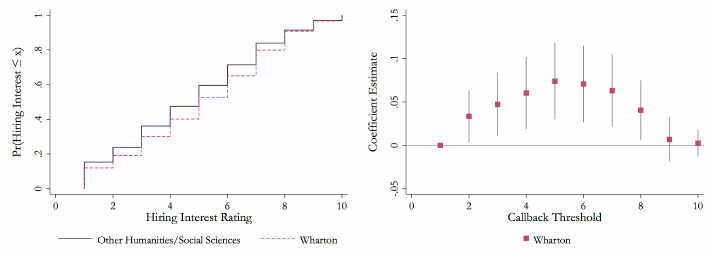
Figure B.1: Wharton
(a) Empirical CDF (b) Linear Probability Model
Empirical CDF of Hiring Interest (Panel B.1a) and di↵erence in counterfactual call b a ck rates (Panel
B.1b)forWharton and Other Humanities & Social Sciences. Empirical CDFs show the share of
hypothetical candidate resumes with each characteristic with a Hiring Interest rating less than or
equal to each value. The counterfactual callback plot shows the di↵erence between groups in the
share of candidates at or above the threshold—tha t is, the share of candidates who would be called
back in a resume audit study if the c a ll b ack threshold were set to any given value. 95% confidence
intervals are calculated from a linear probability mode l with an indicator for being at or above a
threshold as the dependent variable.
73
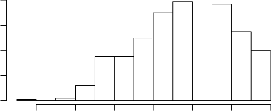
Figure B.2: Distribution of GPA Among Scrap e d Resumes
GPA
Frequen cy
2.8 3.0 3.2 3.4 3.6 3.8 4.0
0 20 40 60 80
Histogram representing the distribution of GPA among scraped resum es in ou r candidate matching
pool. Distribution excludes any resumes fo r which GPA was not available (e.g., resume did not
list GPA, resume listed only GPA within concentration, or parser failed to scrape). GPAs of
participating Penn seniors may not represent the GPA distribution at Penn as a whole.
contend with a limi t ed number of underlying resumes (i.e., resumes that they ma-
nipulate to create treatment variation). Gi ven u n cer t ai nty about the characteristics
of candidates and the limited number of un de rl y i ng resumes, resume auditors may
not be able t o perfec t ly match the distribution of characteristics of a target pop ul a-
tion. An addition al advantage of the IRR methodology is that it involves collecting
a large number of resumes from an applicant pool of real job seekers, which gives
us information on the distribution of candidate characteristics that we can use to
re-weight the data ex post.
74

Table B.3: Human Capital Experience—Weighted by GPA
Dependent Variable: Hiring Interest
OLS OLS OLS
GPA-Scal e d
OLS
Ordered
Probit
GPA 2.274 2.339 2.320 1 0.963
(0.175) (0.168) (0.146) (.) (0.0785)
Top Internship 0.831 0.832 0.862 0.372 0.353
(0.110) (0.109) (0.0882) (0.0428) (0.0474)
Second Internship 0.488 0.482 0.513 0.221 0.216
(0.129) (0.130) (0.105) (0.0475) (0.0545)
Work for Money 0.178 0.193 0.199 0.0856 0.0753
(0.129) (0.125) (0.100) (0.0436) (0.0556)
Technical Skills 0.0768 0.0388 -0.106 -0.0455 0.0224
(0.118) (0.119) (0.102) (0.0439) (0.0507)
Female, White -0.0572 - 0. 0991 -0.0382 -0.0165 -0.0214
(0.134) (0.130) (0.105) (0.0453) (0.0574)
Male, Non-White -0.239 -0.181 -0.111 -0.0480 -0.0975
(0.154) (0.154) (0.123) (0.0530) (0.0658)
Female, Non-White -0.0199 -0.0316 0.0398 0.0171 -0.0175
(0.166) (0.162) (0.134) (0.0577) (0.0710)
Observations 2880 2880 2880 2880 2880
R
2
0.146 0.224 0.505
p-value for test of joi nt
significance of Majors < 0.001 < 0.001 < 0.001 < 0.001 < 0.001
Major FEs Yes Yes Yes Yes Yes
Leadership FEs No Yes Yes Yes No
Order FEs No Yes Yes Yes No
Subjec t FEs No No Yes Yes No
Ordered probit cutpoints: 2.30, 2 . 71 , 3.04, 3.34, 3.66, 3.99, 4.49, 4.95, and 5.46.
Table shows OLS and ordered probit regressions of Hiring Interest from Equation
(1), weighted by the distribution of GPA in resumes in the candi d ate m at ching pool.
Robust standard errors are reported in parentheses. GPA; Top Internship; Second
Internship; Work for Money; Technical Skills; Female, White; Male, Non-White;
Female, Non-White and major are characteristics of the hypothetical resume, con-
structed as descri bed in Section 2.3 and in Appendix A.2. Fixed e↵ects for major,
leadership experience, resume order, and subject i nc l ud ed in some specifications as
indicated. R
2
is indicated for each OLS regression. GPA-Scaled OLS presents the
results of Column 3 d i vi d ed by the Column 3 coefficient on GPA, with standard
errors calculated by delta method. The p-value of a test of joint significance of
major fixed e↵ects is indicated for each model (F -test for OLS regressions,
2
test
for ordered probit regression).
75

Table B.4: Human Capital Experience by Major Type—Weighted by GPA
Dependent Variable: Hiring Interest
Humanities & Social Sciences STEM
OLS OLS OLS
GPA-Scal e d
OLS
Ordered
Probit OLS OLS OLS
GPA-Scal e d
OLS
Ordered
Probit
GPA 2.365 2.452 2.476 1 1.008 2.028 2.187 2.000 1 0.848
(0.212) (0.198) (0.172) (.) (0.0964) (0.306) (0.325) (0.266) (.) (0.133)
Top Internship 0.973 0.941 0.982 0.397 0.412 0.448 0.526 0.581 0.291 0.204
(0.127) (0.125) (0.102) (0.0486) (0.0557) (0.218) (0.222) (0.182) (0.101) (0.0927)
Second Internship 0.476 0.384 0.494 0.199 0.217 0.529 0.496 0.383 0.192 0.223
(0.153) (0.155) (0.125) (0.0520) (0.0645) (0.235) (0.252) (0.199) (0.103) (0.102)
Work for Money 0.0914 0.0349 0.0861 0.0348 0.0366 0.387 0.459 0.517 0.259 0.182
(0.152) (0.145) (0.118) (0.0477) (0.0653) (0.247) (0.270) (0.201) (0.106) (0.106)
Technical Skills 0.0893 0.0263 -0.146 -0.0591 0.0258 0.0111 -0.0591 -0.0928 -0.0464 0.00518
(0.142) (0.142) (0.120) (0.0484) (0.0609) (0.217) (0.240) (0.193) (0.0965) (0.0932)
Female, White 0.110 0. 0360 0.110 0.0445 0.0475 -0.460 -0.637 -0.658 -0.329 -0.183
(0.159) (0.153) (0.125) (0.0506) (0.0683) (0.251) (0.253) (0.206) (0.110) (0.107)
Male, Non-White -0.0332 0.0366 0.0377 0.0152 -0.00558 -0.799 -0.704 -0.590 -0.295 -0.352
(0.181) (0.183) (0.147) (0.0593) (0.0767) (0.295) (0.322) (0.260) (0.129) (0.130)
Female, Non-White 0.0356 0.0238 0.0785 0.0317 0.00129 -0.180 0.0136 0.0391 0.0196 -0.0743
(0.189) (0.186) (0.154) (0.0623) (0.0819) (0.332) (0.318) (0.264) (0.132) (0.140)
Observations 2040 2040 2040 2040 2040 840 840 840 840 840
R
2
0.141 0.242 0.522 0.150 0.408 0.644
p-value for test of joi nt
significance of Majors 0.105 0.152 0.022 0.022 0.138 < 0.001 0.003 < 0.001 < 0.001 < 0.001
Major FEs Yes Yes Yes Yes Yes Yes Yes Yes Yes Yes
Leadership FEs No Yes Yes Yes No No Yes Yes Yes No
Order FEs No Yes Yes Yes No No Yes Yes Yes No
Subjec t FEs No No Yes Yes No No No Yes Yes No
Ordered probit cutpoints (Column 5): 2.54, 2.89, 3.23, 3. 5 4, 3.86, 4.20, 4.71, 5.18, 5.70.
Ordered probit cutpoints (Column 10): 1.78, 2.31, 2.62, 2 . 89 , 3.20, 3.51, 3.98, 4.44, 4.92.
Table shows OLS and ordered probit regressions of Likelihood of Acceptance from Equation (1). GPA; Top Internship ; Second Internship; Work for Money;
Technical Skil ls ; Female, White ; Male, Non-White; Female, Non-White and major are characteristics of the hypothetical resume, cons t ru ct ed as described in
Section 2.3 and in Appendix A.2. Fixed e↵ects for major, leadership experience, resume order, and subject included as indicated. R
2
is indicated for each OLS
regression. GPA-Scaled OLS columns present the res u lt s of Column 3 and Colu mn 8 divided by the Column 3 and Column 8 co effic i ent on GPA, with standard
errors calculated by delta method. The p-values of tests of joint significance of major fixed e↵ect s and demographic va ria b l es are indicated (F -test for OLS,
likelihood ratio test for ordered probit) after a Bonferroni correction for an al y z ing two subgroups.
76

B.3 Distributional Appendix
As discussed in Section 3.3, average preferences for candidate characteristics
might di↵er from the preferences observed in the tails. The stylized example in
Figure B.3 shows this concern graphically. Imagine the light (green) distribution
shows the expect ed prod uc ti v i ty—based on the content of their resumes—of un-
dergraduate research assistants (RAs) majoring in Economics at the University of
Pennsylvania and the dark (gray) distribution shows the expected productivity of
undergraduate RAs enrolled at the Whart on School. In this example, the mean
Wharton student would make a less productive RA, reflecting a lack of interest in
academic research relative to business on average; however, the tails of the Whar-
ton distribution are fatter, reflecting the f act that admission into Wharton is more
selective, so a Wharton student wh o h as evi d en ce of research interest on her resume
is expected to be bett e r than an Economics student with an otherwise identical
resume. Looking across the panels in Fi gur e B.3, we see that as callback thresholds
shift from being high (pan el (a), where professors are very selective, only calling
back around 8% of resu mes ) to medium (panel (b), where professors are calling
back around 16% of resumes) to low (panel (c), where professors are calling back
around 28% of resumes), a researcher conducting a resume audit study might con-
clude that there is an advantage on the RA market of being at W har t on , no e↵ect,
or a disadvantage.
41
A researcher might particularly care about how employers respond to candidate
characteristics around the empirically observed threshold (e.g., the researcher may
be particularly interested in how employers respond to candidates in a particular
market, with a particular level of selectivity, at a particular point in time). Never-
theless, there are a number of reasons why richer inf orm at ion about the underlying
distribution of employer preferences for characteristics would be valuable for a re-
searcher to uncover. A researcher might want to know h ow sensitive estimates are
to: (1) an economic expansion or contraction that changes firms’ hiring needs or
(2) new technologies, such as video conferencing, which may change the callback
threshold by changing the costs of interviewing. Similarly, a res ear cher may be in-
terested in how candidate characteristics would a↵ect callback in di↵erent markets
41
This stylized example uses two normal distributions. In settings where distributions are less
well-behaved, the di↵erence in callback rates might be even more sensitive to specific thresholds
chosen.
77

Table B.5: Likelihood of Acceptance—Weighted by GPA
Dependent Variable:
Likelihood of Acceptance
OLS OLS OLS
Ordered
Probit
GPA 0.545 0.552 0.663 0.246
(0.174) (0.168) (0.132) (0.0738)
Top Internship 0.725 0.709 0.694 0.299
(0.111) (0.108) (0.0833) (0.0472)
Second Internship 0.524 0.456 0.432 0.220
(0.132) (0.133) (0.101) (0.0556)
Work for Money 0.205 0.150 0.185 0.0872
(0.128) (0.125) (0.0977) (0.0544)
Technical Skills 0.0409 -0.0390 -0.114 0.0122
(0.120) (0.120) (0.0972) (0.0504)
Female, White -0.209 -0.276 -0.224 -0.0830
(0.135) (0.133) (0.103) (0.0571)
Male, Non-White -0.248 -0.273 -0.114 -0.113
(0.157) (0.155) (0.120) (0.0660)
Female, Non-White -0.174 -0.224 -0.155 -0.0856
(0.160) (0.156) (0.124) (0.0684)
Observations 2880 2880 2880 2880
R
2
0.077 0.162 0.509
p-value for test of joi nt
significance of Majors < 0.001 < 0.001 < 0.001 < 0.001
Major FEs Yes Yes Yes Yes
Leadership FEs No Yes Yes No
Order FEs No Yes Yes No
Subjec t FEs No No Yes No
Ordered probit cutpoints: -0.09, 0.29, 0.64, 0.90, 1.26, 1.67, 2.13, 2.65, and 3 .0 2 .
Table shows OLS and ordered probit regressions of Likelihood of Ac-
ceptance from Equation (1), weighted by the distribut i on of GPA in
resumes in our candidate matching pool. Robust standard errors are re-
ported in parentheses. GPA; Top Internshi p; Second Internship; Work
for Money; Technical Skills; Female, White; Male, Non-White; Fem al e,
Non-White are characteristics of the hypothetical resume, constructed
as described in Section 2.3 and in Appendix A.2. Fixed e↵ects for ma-
jor, leadership experience, resume ord er , and subject included in some
specifications as indicated. R
2
is indicated for each OLS regression. The
p-value of a test of joint significance of major fixed e↵ects i s indicated
(F - t est for OLS regressions,
2
test for ordered probit regression) .
78
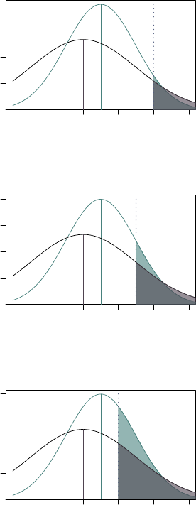
Figure B.3: Callback Thresholds Example
0 2 4 6 8 10
0.05 0.10 0.15 0.20
Value
Density
6.68%
9.12%
(a) High Threshold
0 2 4 6 8 10
0.05 0.10 0.15 0.20
Value
Density
15.9%
15.9%
(b) Medium Threshold
0 2 4 6 8 10
0.05 0.10 0.15 0.20
Value
Density
30.9%
25.2%
(c) Low Threshold
A stylized example where average preferences di↵er from preferences at the upper tail . The distri-
bution in green has a higher mean and lower variance, leading to thinner tails; the distribution in
gray has a lower mean but higher variance, leading to more mass in the upper tail. As the callback
threshold decreases from Panel (a) to Panel (c ) , the share of candidates above the threshold from
each distribution changes. Estimating preferences from callbacks following this type of threshold
proc ess might lead to spurious conclusio ns .
79
(e.g., those known to be more or less selective) than the market where a resume
audit was conducted. To conduct these counterfactual analyses, richer preference
information would be valuable.
B.3.1 Comparing Results Across the Distribution
Resume aud it studies often report di↵e re nc es in callback rates b etween two types
of job candidates, either in a t-test or in a regression. However, as the overall callback
rate becomes very large (i.e., almost all candidates get called back) or very small
(i.e., few candidates get called back), the di↵erence s in callb ack rates tend toward
zero. This is because, as discussed in foot n ot e 22, the maximum possible di↵erence
in callback rates is capped by the overall callback rate.
This i s not a threat t o the internal validity of most resume audit studies executed
in a single hiring environment. However, this can cause p rob l ems when comparing
across studies, or within a st udy run in di↵erent environments. For example, if one
wanted to show that there was less racial discrimination in one city versus another,
and the underlying callback rates in those cities di↵ered, an interaction between
city and race may be difficult to interpret. Note that such an exerci s e is performed
in Kroft et al. [ 2013] to compare the response to unemployment in cities with high
unemployment (and likely low overall callback rates) versus ci t ie s with low unem-
ployment rates (and high callback rates). In that particular study, the “bias” caused
by comparing across di↵er e nt callback rates does not undermine the finding that
high unemployment rate cit i es respond less to unemployment spells. Nonetheless,
researchers should use caution when implementing similar study designs.
In Figures B.4 and B.5, we look at how two di↵erent ways of measuring call-
back di↵erences perform across the distribution compared to the linear probability
model. The lefthand side of each figure shows the ratio of the callback rates, another
common way of reporting resume audit study results. For the positive e↵ects in our
study, this odds ratio tends to be larger at the upper tai l , where a small di↵erence
in callbacks can result in a large response in the ratio. On the righthand side of
each figure, we show e↵ects estimated from a logit specification. We find that in our
data, the e↵ects estimated in logistic regression tend to be flatt e r across the quality
distribution.
80
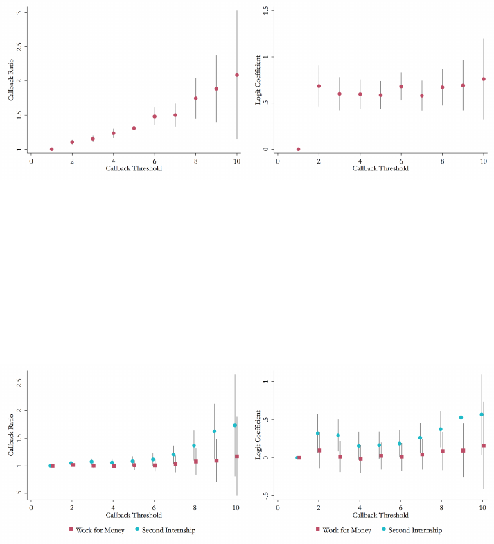
Figure B.4: Alternative Specificat i on s: Top Internship
(a) Callback Ratio (b) Logit
Counterfactual callback ratios (Panel B.4a) and counterfactual logit coefficients (Panel B.4b) for
Top Internship. Counterfactual callback is an indicator for each value of Hiring Interest equal
to 1 if Hiring Interest is greater than or equal to the value, and 0 otherwise. Callback ratio is
defined as the counterfactual callback rate for candid a t es with the characteristic divided by the
counterfactual callback rate for candidates without. 95% confidence intervals are calculated from
a linear probability model using the delta method. Logit coefficients are estimated from a logit
regression with counterfactual callback as the dep en d ent variable.
Figure B.5: Alternative Specificat i on s: Second Job Type
(a) Callback Ratio (b) Logit
Counterfactual callback ratios (Panel B.5a) and counterfactual logit coefficients (Panel B.5b) for
Work for Money and Second Internship. Counterfactual callback is an indicator for each value of
Hiring Interest equal to 1 if Hiring Interest is greater than or equal to the value, and 0 otherwise.
Callback ratio is defined as the counterfactual callback rate for candidates with the characteristic
divided by the counterfactual callback rate for candidates without. 95% confidence intervals are
calculated from a linear probability model using the delta method. Logit coefficients are estima ted
from a logit regression with counterfactual callba ck as the dependent varia b le.
81

B.4 Candidate Demographics Appendix
In this section, we provide additional analyses for our main results on candidate
demographics. In B.4.1, we analyze our findings by t h e demographics of employers
evaluating resumes. In B.4.2 we describe a test for implicit bias. In B.4.3,wediscuss
di↵erential returns to quality by demographic group.
B.4.1 Rater Demographics
IRR allows us to collect information about the spe ci fic individuals rating resumes
at the hiring firm. In Table B.6 we explore our main results by rater gen de r and race.
White and female raters appear more likely to discriminate against male, non-white
candidates than non-white or female raters.
B.4.2 Test for Implicit Bias
We leverage a feature of implicit bias—that it is more likely to arise when decision
makers are fatigued [Wigboldus et al., 2004, Govoru n and Payne, 2006, Sherman
et al., 2004]—to test whether our data are consistent with implicit bias. Appendix
Table B.7 investigates how employers respond to resumes in the first and second
half of the study and to resumes before an d after the period breaks—after every 10
resumes—that we built into the survey tool.
42
The first and second columns show
that subjects spend less time evaluating each resume in th e second half of the stud y
and in the latter half of each block of 10 resumes, suggesting evidence of fatigue.
The third col um n reports a statistically significant interaction on Latter Half of
Block ⇥ Not a White Male of 0.385 Likert-scale points, equi valent to about 0.18
GPA points, suggesting more discrimination against candidates who are not white
males in the latter half of each block of 10 resumes. The fourth column reports,
however, t hat the bias in the second half of th e study is not statistically significantly
larger than the bias i n the first half. These re su l ts provide suggestive, though not
conclusive, evidence that the discrimination we detect may indeed be driven by
implicit bias.
42
As described i n Section 2, after every 10 resumes an employer completed, the employer was
shown a simple webpage with an affirmation that gave them a short break (e.g., after the first 10
resumes it read: “You have rated 1 0 of 40 resumes. Keep up th e good work!”). Research suggests
that such “micro breaks” can have relatively large e↵ects on focus and attention [Rzeszotarski et al.,
2013], and so we compare bias in the early half and lat t er half of each block of 10 resumes under the
assumption t h a t employers might be more fatigued in the latter half o f each block of 10 resumes.
82

Table B.6: Hiring Interest by Rater Demographics
Dependent Variable: Hire Rating
Rater Gender Rater Race
All
Female
Raters
Male
Raters
Non-White
Raters
White
Raters
GPA 2.196 2.357 2.092 2.187 2.131
(0.129) (0.170) (0.212) (0.378) (0.146)
Top Internship 0.897 0.726 1.139 1.404 0.766
(0.0806) (0.105) (0.140) (0.234) (0.0914)
Second Internship 0.466 0.621 0.195 0.636 0.459
(0.0947) (0.126) (0.154) (0.273) (0.107)
Work for Money 0.154 0.303 -0.0820 -0.124 0.192
(0.0914) (0.120) (0.156) (0.255) (0.104)
Technical Skills -0.0711 -0.0794 -0.0202 -0.123 -0.0164
(0.0899) (0.122) (0.151) (0.231) (0.104)
Female, White -0.161 -0.202 -0.216 0.00413 -0.209
(0.0963) (0.128) (0.165) (0.265) (0.109)
Male, Non-White -0.169 -0.311 -0.105 0.119 -0.241
(0.115) (0.149) (0.200) (0.285) (0.132)
Female, Non-White 0.0281 0.00110 -0.0648 -0.124 0.0968
(0.120) (0.159) (0.202) (0.325) (0.137)
Observations 2880 1720 1160 600 2280
R
2
0.483 0.525 0.556 0.588 0.503
Major FEs Yes Yes Yes Yes Yes
Leadership FEs Yes Yes Yes Yes Yes
Order FEs Yes Yes Yes Yes Yes
Subject FEs Yes Yes Yes Yes Yes
OLS regressions of Hiring Interest on candidate characteristics by rater gender and race.
Sample includ es 29 male and 42 female subjects; 57 White and 15 non-White subjects. Ro-
bust standard errors are reported in parentheses. GPA; Top Internship ; Second Internship;
Work for Money; Technical Skil ls ; Female, White ; Male, Non-White; Female, Non-White
are characteristics of the hypothetical resume, constructed as described in Section 2.3 and in
Appendix A.2. R
2
is indicated for each OLS regression. Fixed e↵ects for major, leadership
experien c e, resume order, and subject inc l u d ed in some specificat io n s as indicated.
83

Table B.7: Implicit Bias
Dependent Variable:
Response Time
Dependent Variable:
Hiring Interest
Latter Half of Block -3.518 0.360
(0.613) (0.137)
Second Half of Study -4.668 -0.142
(0.598) (0.138)
Not a White Male -0.642 -0.648 0.0695 -0.107
(0.666) (0.665) (0.115) (0.118)
Latter Half of Block ⇥
Not a White Male -0.385
(0.165)
Second Half of Study ⇥
Not a White Male -0.0225
(0.166)
GPA 2.791 2.944 2.187 2.187
(0.961) (0.949) (0.128) (0.128)
Top Internship -0.799 -0.638 0.905 0.904
(0.622) (0.620) (0.0802) (0.0800)
Second Internship 2.163 2.118 0.471 0.458
(0.752) (0.750) (0.0934) (0.0934)
Work for Money 1.850 1.813 0.154 0.140
(0.741) (0.740) (0.0909) (0.0910)
Technical Skills 0.881 0.892 -0.0668 -0.0780
(0.715) (0.713) (0.0889) (0.0890)
Observations 2880 2880 2880 2880
R
2
0.405 0.412 0.475 0.475
p-value for test of joi nt
significance of Majors < 0.001 < 0.001 < 0.001 < 0.001
Major FEs Yes Yes Yes Yes
Leadership FEs Yes Yes Yes Yes
Order FEs No No No No
Subject FEs Yes Yes Yes Yes
Regressions of Response Time and Hiring Interest on resume characteristics and re-
sume order variables. The first and s ec on d columns show Response Time regressions;
the third and fo u rt h columns show Hiring Interest regressions. Response Time is
defined as the number of seconds before page submission, Winsorized at the 95
th
per-
centile (77.9 seconds). Mean of Response Time :23.6seconds.GPA, Top Internship,
Second Internship, Work for Money, Technical Skil ls,andNot a White Male are char-
acteristics of the hypothetical resume, constructed as described in Section 2.3 and in
Appendix A.2. Latter Half of Block is an indicator variable for resumes shown among
the last five resumes within a 10-resume block. Second Half of Study is an indicator
variable for resumes shown among th e last 20 resumes viewed by a subject. Fixed
e↵ects for subjects, majors, and leadership experience included in all sp ec i fi ca t i on s .
R
2
is indicated for each OLS regression. The p-value of an F test of joint significance
of major fixed e↵ects is indicated for all models.
84
B.4.3 Interaction of Demograp h i cs with Qu al ity
Table B.8 shows that whi te males gain more from having a Top Internship than
candidates who are not white males. The largest of these coeffic ie nts, that for non-
white females, nearly halves the benefit of having a prestigious internship. We spec-
ulate that this may b e due to firms believing that prestigious internships are a less
valuable signal of quality if the previous employer may have selected the candidate
due to positive tastes for diversity. Figure B.6 looks at th e relationship between Top
Internship and being Not a White Male th r ough out t he qu ali ty distribution. We
find that when a candidate is of sufficiently high quality, a Top Internship i s equally
valuable for white male candidates and those who are n ot white males. This may
suggest that other signals of quality may inoculate candidates from the assumption
that an impressive work history is the result of diversity initiatives.
85

Table B.8: Return to Top Internship by Demographic Group
Dependent Variable: Hiring Interest
OLS OLS OLS
GPA-Scal e d
OLS
Ordered
Probit
GPA 2.119 2.184 2.191 1 0.889
(0.145) (0.150) (0.129) (.) (0.0613)
Top Internship 1.147 1.160 1.155 0.527 0.471
(0.168) (0.175) (0.145) (0.0736) (0.0704)
Second Internship 0.468 0.495 0.470 0.214 0.208
(0.112) (0.118) (0.0944) (0.0446) (0.0469)
Work for Money 0.109 0.151 0.148 0.0675 0.0496
(0.110) (0.113) (0.0913) (0.0417) (0.0469)
Technical Skills 0.0494 0.0576 -0.0670 -0.0306 0.0132
(0.104) (0.108) (0.0899) (0.0411) (0.0442)
Female, White 0.0327 -0.0188 0.0225 0.0103 0.0118
(0.146) (0.152) (0.121) (0.0554) (0.0617)
Male, Non-White -0.0604 -0.0488 -0.0553 -0.0253 -0.0287
(0.175) (0.184) (0.145) (0.0659) (0.0741)
Female, Non-White 0.0806 0.0685 0.159 0.0727 0.0104
(0.182) (0.191) (0.156) (0.0717) (0.0768)
Top Internship ⇥
Female, White -0.464 -0.492 -0.459 -0.209 -0.181
(0.234) (0.243) (0.199) (0.0920) (0.0974)
Top Internship ⇥
Male, Non-White - 0.280 -0.316 -0.276 -0.126 -0.116
(0.279) (0.288) (0.233) (0.107) (0.116)
Top Internship ⇥
Female, Non-White -0.229 -0.224 -0.316 -0.144 -0.0653
(0.273) (0.286) (0.240) (0.110) (0.116)
Observations 2880 2880 2880 2880 2880
R
2
0.130 0.182 0.484
p-value for test of joi nt
significance of Majors < 0.001 < 0.001 < 0.001 < 0.001 < 0.001
Major FEs Yes Yes Yes Yes Yes
Leadership FEs No Yes Yes Yes No
Order FEs No Yes Yes Yes No
Subjec t FEs No No Yes Yes No
Ordered probit cutpoints: 1.94, 2 . 31 , 2.68, 2.97, 3.29, 3.63, 4.09, 4.55, and 5.06.
Table shows OLS and ordered probit regr ess i ons of hiring interest from Equation
(1). Robust standard errors are reported in parentheses. GPA; Top Interns hi p;
Second Internship; Work for Money; Technical Skills; Female, White; Male, Non-
White; Female, Non-White are characteristics of the hypothetical resume, con-
structed as descri bed in Section 2.3 and in Appendix A.2. Fixed e↵ects for major,
leadership experience, resume order, and subject i nc l ud ed in some specifications as
indicated. R
2
is indicated for each OLS regression. GPA-Scaled OLS presents the
results of Column 3 d i vi d ed by the Column 3 coefficient on GPA, with standard
errors calculated by delta method. The p-value of a test of joint significance of
major fixed e↵ects is indicated (F -test for OLS, likelihood ratio test for ordered
probit).
86
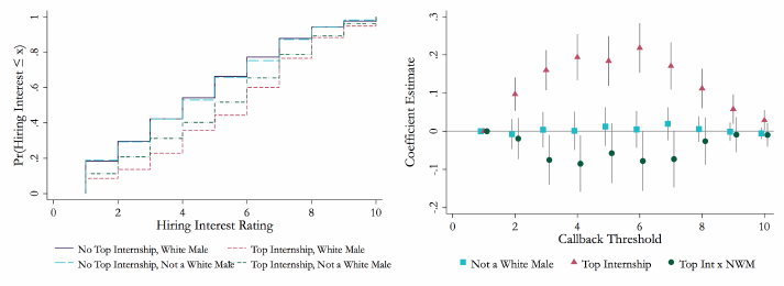
Figure B.6: Top Internship ⇥ Not a White Male
(a) Empirical CDF (b) Linear Probability Model
Empirical CDF of Hiring Interest (Panel B.6a) and di↵erence in counterfactual callback rates
(Panel B.6b) for Top Internship, Not a White Male,andTop Internship ⇥ Not a White Male.
Empirical CDF s show the share of hypo t h eti c a l candidate resumes with each characteristic with a
Hiring Interest rating less than or equal to each value. The counterfactual callback plo t shows the
di↵erence between groups in the share of candidates at or above the threshold—th a t is, the share
of candidates who would be called back in a resume audit study if the callback threshold were set
to any given value. 95% confidence intervals are calc u la t ed from a linear probability model with an
indicator fo r being at or above a threshold as the dependent variable.
B.5 Relationship Between Likelihood of Acceptance and Human
Capital
In evaluating candidates’ likelihood of accepting a job o↵er, the firms in our
sample exhibit a potentially surprising belief that candidates with more human
capital—indicated by h igh er GPA, more work experience, and a more prestigious
internship—are more likely to accept jobs than candidates with less human capital.
This correlation could arise in several ways. First, it is possible that the hiring inter-
est question—which always comes firs t —c re at e s anchoring for the second question
that is unrelated t o true beliefs. Second, it is possible that li kelihood of acceptance
is b ased on both horizontal fit and vertical quality. Horizontal fit raises both hiring
interest and likelihood of acceptance, which would lead to a positive correlation be-
tween responses; vertical quality, on the other hand, would be expected to increase
87

hiring interest and decrease likelihood of acceptance, since as it incr eas es hiring
interest it al s o makes workers more desirable for other firms.
43
If the correlation between Hiring Interest and Likelihood of Acceptance is driven
mostly by horizontal fit, it is important to test whether Likelihood of Acceptance
is simply a noisy measure of Hiring Interest, or whether Likelihood of Acceptance
contains additional, valuable information. This will help us confirm, for example,
that the gender bias we find in Likelihood of Acceptance is indeed its own result,
rather than a result of bias in Hiring Interest. Approaching this is econometrically
tricky, since Hiring Interest and Likelihood of Acceptance are both simultaneous
products of the rater’s assessment of the randomized resume components. We con-
sidered multiple approaches, such as subtr act i ng hiring interest from likeliho od of
acceptance to capture the di↵erence, regressing likelihood of acceptance on hiring
interest and taking residuals, and including controls for hiring interest. All yield
similar results, and so we use the latter approach, as it is the most transparent.
Despite its econometric issues, we believe this is nonetheless a helpful exercise that
can be thought of as akin to a mediation analysis. We want to see if all of the
e↵ect on Likelihood of Acceptance is mediated through Hiring Interest, or if there is
independent variation in Likelihood of Accept ance.
The first two columns of Table B.9 include a linear control for Hiring Interest,
while Columns 3 and 4 inclu de fixed e↵ect controls for each level of the Hiring
Interest rating, examining Likelihood of Acceptance within each hiring interest band.
We find that after controlling for Hiring interest, the relationship between GPA
and Likelihood of Acceptance becomes negative and statistically significant under
all specifications. This indicates that the part of Likelihood of Acceptance that is
uncorrelated with Hiring Interest is indeed negatively correlated with one measure
of vertical quality. We also find that the coefficients on Top Internship and Second
Internship become stati st i cal l y indistinguishable from zero.
Under all specifications, the coefficients on Female, White and Female, Non-
White remain negative and significant, indicating that employers believe women are
43
It is al so possible that respondents deliberately overstate candidates’ likelihood of acceptance
in order to be sent the best quality candidates. However, firms who are willing to do this likely
have a low cost of interviewing candidates with a lower probability of acceptance. This is in line
with the data, where the firms who consistently rate people a 10 on Likelihood of Acceptance are
among the most prestigious firms in our sample.
88
less likely to accept jobs if o↵ered, even controlling for the firm’s interest in the
candidate.
Thus, we conclude that Likelihood of Acceptance does provide some additional
information above and beyond Hiring Interest. We hope future research will tackle
the question of how to measure beliefs about Likelihood of Acceptance accurately,
how to disentangle the m from Hiring Interest, and exactly what role they play in
hiring decisions.
89

Table B.9: Likelihood of Acceptance with Hiring Interest Controls
Dependent Variable:
Likelihood of Acceptance
OLS
Ordered
Probit OLS
Ordered
Probit
GPA -0.812 -0.638 -0.823 -0.660
(0.0820) (0.0641) (0.0815) (0.0646)
Top Internship 0.0328 0.000290 0.0313 0.000698
(0.0535) (0.0406) (0.0534) (0.0408)
Second Internship 0.0656 0.0511 0.0680 0.0491
(0.0634) (0.0477) (0.0634) (0.0480)
Work for Money 0.0951 0.0824 0.0954 0.0868
(0.0611) (0.0475) (0.0610) (0.0477)
Technical Skills -0.0527 -0.0572 -0.0608 -0.0661
(0.0596) (0.0449) (0.0594) (0.0452)
Female, White -0.145 -0.0781 -0.147 -0.0820
(0.0638) (0.0484) (0.0638) (0.0486)
Male, Non-White 0.00212 -0.0162 0.000650 -0.00832
(0.0744) (0.0577) (0.0744) (0.0580)
Female, Non-White -0.182 -0.154 -0.185 -0.159
(0.0741) (0.0587) (0.0737) (0.0591)
Hiring Interest 0.704 0.478 FEs FEs
(0.0144) (0.0104)
Observations 2880 2880 2880 2880
R
2
0.766 0.768
p-value for test of joi nt
significance of Majors 0.025 < 0.001 0.031 < 0.001
Major FEs Yes Yes Yes Yes
Leadership FEs Yes No Yes No
Order FEs Yes No Yes No
Subjec t FEs Yes No Yes No
Cutpoints (Col 2): -1.82, -1.18, -0.5 5, -0.11, 0.49, 1.07, 1.71, 2.39, 2.81.
Cutpoints (Col 4): -2.00, -1.26, -0.5 8, -0.14, 0.45, 1.01, 1.62, 2.28, 2.69.
Table shows OLS and ordered p ro b it regressions of Likelihood of Acceptance from
Equation (1), with add it io n a l controls for Hiring Interest. Robu st standard errors
are reported in parentheses. GPA; Top Internship ; Second Internship; Work f or
Money; Technical Skil ls ; Female, White ; Male, Non-White; Female, Non-White
and major are characteristics of the hypothetical resume, c o n st ru c te d as described
in Section 2.3 and in Appendix A.2. Fixed e↵ects for major, leadership experi en c e,
resume order, and subject included in some specifications as indicated. R
2
is indi-
cated for each OLS regression. The p-values of tests of joint significance of major
fixed e↵ects and demographic variables are indicated (F -test for OLS, likelihood
ratio test for ordered p ro b i t ).
90
C Pitt Appendix
In our replication study at the University of Pittsburgh, we followed a similar
approach to that described for our experimental waves at Penn i n Section A.2.The
tool structure was essentially the same as at Penn, with references to Penn replaced
with Pitt in the instructions, and the reference to Wharton removed from th e major
selection page. Resume structure was identical to that described in Sections A.2.1
and A.2.2. Names were randomized in the same manner as described in Section
A.2.3. The education section of each resume at Pitt followed the same structure as
that described in Section A.2.4, but had a degree from the University of Pittsburgh,
with majors, schools, and degrees randomly drawn from a set of Pitt’s o↵erings.
In selecting majors for our Pitt replication, we attempted to match the Penn ma-
jor distribution as closely as possible, but some majors were not o↵ered at both
schools. When necessary, we selected a similar major instead. The maj or s, schools,
classifications, and probabilities for Pitt are shown in Table C.1.
We used a single pool of Pitt resumes for both the hypothe t i cal resume elements
and for a candidate pool for Pitt employers, saving si gn i fic ant e↵ort on scraping and
parsing. These components were compiled and randomized in much the same way
as at Penn, as described in Section A.2.5. For Top Internship at Pitt, we collected
work experiences from Pi t t resumes at one of Pitt’s most fre q ue nt employers, or at
one of the employers used to define Top Internship at Penn. Similarly, Pitt Work
for Money was identified from th e same list of identifying phrases shown in Table
A.5. Technical Skills were randomized in the same way as at Penn, described in
A.2.5.
91

Table C.1: Majors in Generated Pitt Resumes
Type School Major Probability
Humanities &
Social Sciences
Dietrich School of
Arts and Sciences
BS in Economics 0.4
BA in Economics 0.2
BS in Political Science 0.075
BS in Psychology 0.075
BA in Communication Science 0.05
BA in English Literature 0.05
BA in History 0.05
BA in History of Art and Architecture 0.025
BA in Philosophy 0.025
BA in Social Sciences 0.025
BA in Sociology 0.025
STEM
Dietrich School of
Arts and Sciences
BS in Natural Sciences 0.1
BS in Molecular Biology 0.075
BS in Bioinformatics 0.05
BS in Biological Sciences 0.05
BS in Chemistry 0.05
BS in Mathematical Biology 0.05
BS in Mathematics 0.05
BS in Physics 0.05
BS in Statistics 0.025
Swanson School of
Engineering
BS in Computer Engineering 0.15
BS in Mechanical Engineering 0.075
BS in Bioengineering 0.05
BS in Chemical Engineering 0.05
BS in Computer Science 0.05
BS in Electrical Engineering 0.05
BS in Materials Science and Engineeri ng 0.05
BS in Civil Engineering 0.025
Majors, degrees, schools within Pitt, and their selection probability by major type. Majors (and
their associated degrees and schools) were drawn with replacement and randomized to resumes
after subjects s elec t ed to view either Humanities & Social Sciences resumes or STEM resumes.
92

Table C.2: E↵ects by Major Type at Pitt
Dependent Variable: Hiring Interest
Humanities & Social Sciences STEM
OLS OLS OLS
GPA-Scal e d
OLS
Ordered
Probit OLS OLS OLS
GPA-Scal e d
OLS
Ordered
Probit
GPA 0.249 0.294 0.249 1 0.0969 0.518 0.445 0.340 1 0.167
(0.189) (0.203) (0.150) (.) (0.0731) (0.245) (0.274) (0.187) (.) (0.0925)
Top Internship 0.267 0.290 0.298 1.196 0.0985 0.164 0.193 0.174 0.513 0.0579
(0.139) (0.150) (0.108) (0.834) (0.0531) (0.156) (0.174) (0.110) (0.419) (0.0602)
Second Internship 0.438 0.496 0.446 1.791 0.169 -0.0224 -0.0758 -0.0825 -0.243 -0.00184
(0.146) (0.154) (0.112) (1.163) (0.0567) (0.184) (0.204) (0.133) (0.414) (0.0718)
Work for Money 0.323 0.354 0.355 1.425 0.121 -0.0629 -0.0391 -0.0369 -0.109 -0.00114
(0.145) (0.155) (0.109) (0.958) (0.0569) (0.186) (0.207) (0.129) (0.386) (0.0720)
Technical Skills -0.0140 -0.0357 0.0372 0.149 -0.00419 0.376 0.459 0.283 0.834 0. 153
(0.131) (0.143) (0.103) (0.418) (0.0507) (0.179) (0.199) (0.129) (0.611) (0.0670)
Female, White -0.0796 -0.177 -0.0434 -0.174 -0.0211 -0.0435 0.0334 0.0492 0.145 -0.0126
(0.149) (0.160) (0.113) (0.467) (0.0579) (0.184) (0.203) (0.133) (0.395) (0.0720)
Male, Non-White 0.0893 0.0368 -0.155 -0.621 0.0435 -0.0448 0.0282 0.0835 0.246 -0.0412
(0.175) (0.189) (0.130) (0.634) (0.0676) (0.232) (0.259) (0.160) (0.481) (0.0893)
Female, Non-White -0.196 -0.331 -0.0732 -0.294 -0.0720 -0.160 -0.0550 0.0906 0.267 -0.0362
(0.180) (0.193) (0.140) (0.592) (0.0689) (0.225) (0.258) (0.160) (0.482) (0.0891)
Observations 2000 2000 2000 2000 2000 1440 1440 1440 1440 1440
R
2
0.015 0.078 0.553 0.031 0.109 0.651
p-value for test of joi nt
significance of Majors 0.713 0.787 0.185 0.185 0.821 0.015 0.023 < 0.001 < 0.001 0.014
Major FEs Yes Yes Yes Yes Yes Yes Yes Yes Yes Yes
Leadership FEs No Yes Yes Yes No No Yes Yes Yes No
Order FEs No Yes Yes Yes No No Yes Yes Yes No
Subjec t FEs No No Yes Yes No No No Yes Yes No
Ordered probit cutpoints (Column 5): -0.38, -0.13, 0.19, 0 . 4 2 , 0.68, 0.98, 1.40, 1.88, 2.45.
Ordered probit cutpoints (Column 10): 0.40, 0.61, 0.85, 1 . 02 , 1.16, 1.31, 1.58, 1.95, 2.22.
Table shows OLS an d ordered probit regressions of Hiring Interest from Equation (1). Robust standard errors are reported in parentheses. GPA; Top Internship ;
Second Internship; Work for Money ; Technical Skil ls ; Female, White ; Male, Non-White; Female, Non-White an d major are characteristics of the hypothetical
resume, constructed as described in Section 2.3 and in Appendix A.2. Fixed e↵ects for majo r, leadership experience, resume order, and subject included as
indicated. R
2
is indicated for each OLS regression. The p-values of tests of joint significance of major fi xed e↵ects and demographic variables are indicated (F -test
for OLS, likelihood ratio test for ordered probit ) after a Bonferroni correction for analyzing two subgroups.
93

Table C.3: Likelihood of Acceptance at Pitt
Dependent Variable: Likelihood of Accept anc e
OLS OLS OLS
Ordered
Probit
GPA 0.178 0.161 0.0104 0.0710
(0.148) (0.155) (0.101) (0.0572)
Top Internship 0.233 0.245 0.235 0.0873
(0.103) (0.108) (0.0680) (0.0398)
Second Internship 0.224 0.221 0.199 0.0739
(0.114) (0.119) (0.0768) (0.0447)
Work for Money 0.142 0.143 0.130 0.0504
(0.114) (0.120) (0.0738) (0.0443)
Technical Skills 0.195 0.187 0.111 0.0843
(0.106) (0.110) (0.0700) (0.0403)
Female, White -0.0627 -0.0795 0.0152 -0.0268
(0.115) (0.122) (0.0774) (0.0448)
Male, Non-White -0.000104 -0.0119 -0.0641 -0.0111
(0.139) (0.145) (0.0907) (0.0539)
Female, Non-White -0.198 -0.197 -0.0483 -0.0702
(0.140) (0.147) (0.0904) (0.0549)
Observations 3440 3440 3440 3440
R
2
0.037 0.061 0.643
p-value for test of joi nt
significance of Majors < 0.001 < 0.001 < 0. 001 < 0.001
Major FEs Yes Yes Yes Yes
Leadership FEs No Yes Yes No
Order FEs No Yes Yes No
Subjec t FEs No No Yes No
Ordered probit cutpoints: -0.10, 0.14, 0.38, 0.58, 0.86, 1.08, 1.42, 1.86, and 2 .3 5 .
Table shows OLS and ordered probit regressions of Likelihood of Accep-
tance from Equation (1). Robust standard errors are reported in parenthe-
ses. GPA; Top Internship; Second Internship; Work for Money; Technical
Skills; Female, White; Male, Non-White; Female, Non-White and major are
characteristics of the hypothetical resume, constructed as described in Sec-
tion 2.3 and in Appendix A.2. Fixed e↵ects for major , leadership experience,
resume order, and subject included in some specifications as indicated. R
2
is
indicated for each OLS regression. The p-values of tests of joint significance
of major fixed e↵ects and demographic variables are indicated (F -test for
OLS, likelihood ratio test for ordered probit).
94

Table C.4: Likelihood of Acceptance by Major Type at Pitt
Dependent Variable: Likelihood of Accept anc e
Humanities & Social Sciences STEM
OLS OLS OLS
Ordered
Probit OLS OLS OLS
Ordered
Probit
GPA -0.0641 -0.0437 -0.173 -0.00697 0.499 0.427 0.278 0.155
(0.187) (0.202) (0.127) (0.0735) (0.241) (0.268) (0.181) (0.0913)
Top Internship 0.261 0.248 0.263 0.0971 0.210 0.227 0.214 0.0781
(0.137) (0.149) (0.0914) (0.0535) (0.155) (0.173) (0.112) (0.0596)
Second Internship 0.353 0.435 0.373 0.124 0.0433 -0.0259 -0.0205 0.0201
(0.146) (0.156) (0.0955) (0.0572) (0.183) (0.201) (0.131) (0.0709)
Work for Money 0.271 0.294 0.303 0.0997 -0.0506 -0.0453 -0.0345 -0.00860
(0.144) (0.155) (0.0949) (0.0572) (0.184) (0.205) (0.126) (0.0712)
Technical Skills -0.0125 0.00378 -0.00849 -0.00497 0.521 0.638 0.382 0.214
(0.130) (0.140) (0.0864) (0.0511) (0.178) (0.195) (0.128) (0.0662)
Female, White -0.0639 -0.149 -0.000568 -0.0353 -0.0808 -0.00711 -0.0254 -0.0136
(0.148) (0.159) (0.0969) (0.0584) (0.183) (0.204) (0.136) (0.0711)
Male, Non-White 0.110 0.0600 -0.132 0.0325 -0.152 -0.0799 0.0216 -0.0725
(0.173) (0.185) (0.112) (0.0681) (0.232) (0.259) (0.162) (0.0886)
Female, Non-White -0.138 -0.258 -0.0954 -0.0623 -0.286 -0.218 -0.0310 -0.0678
(0.180) (0.194) (0.118) (0.0694) (0.224) (0.258) (0.158) (0.0882)
Observations 2000 2000 2000 2000 1440 1440 1440 1440
R
2
0.010 0.069 0.666 0.036 0.110 0.654
p-value for test of joi nt
significance of Majors 1.436 1.550 1.061 1.701 0.006 0.016 < 0.001 0.008
Major FEs Yes Yes Yes Yes Yes Yes Yes Yes
Leadership FEs No Yes Yes No No Yes Yes No
Order FEs No Yes Yes No No Yes Yes No
Subject FEs No No Yes No No No Yes No
Ordered probit cutpoints (Column 4): -0.59, -0.34, -0.11, 0.14, 0.47, 0.76, 1.12, 1.59, 2.37.
Ordered probit cutpoints (Column 8): 0.31, 0.56, 0.78, 0. 9 3, 1.12, 1.25, 1.56, 1.96, 2.26.
Table shows OLS and ordered probit regressi o n s of Likelihood of Acceptance from Equation (1). GPA; Top Internship ; Second
Internship; Work for Money; Technical Skil ls ; Female, White ; Male, Non-White; Female, Non-White and major are characteristics
of the hypothetical resume, constructed as described in S e ct i o n 2.3 and in Appendix A.2. Fixed e↵ects for major, leadership
experien c e, resume order, and subject included as indicated. R
2
is indicated for each OLS regressi on . The p-values of tests of joint
significance of major fixed e↵ects and demographic variables are indicated (F -test for OLS, likelihood ratio test for ordered probit)
after a Bonferroni correction for analyzing two subgroups.
95
